Two-Stage Genomic Analysis

Integrating GBLUP with two-stage MET workflows

Overview

This tutorial extends the two-stage MET workflow to include genomic information. By incorporating a genomic relationship matrix (GRM) at Stage 2, we can:

• Obtain genomic estimated breeding values (GEBVs)
• Predict performance of untested genotypes
• Leverage marker information for selection decisions

The key innovation is using GM(geno, Gmat) alongside vcov(RMAT) to combine genomic relationships with properly propagated BLUE uncertainty.

NoteLearning Objectives

• Prepare and align a GRM for Stage 2 analysis
• Fit GBLUP models using GM() with vcov(RMAT)
• Use the mandala_gp() wrapper for streamlined genomic prediction
• Extract and compare GEBVs from different approaches
• Understand when genomic prediction adds value

ImportantPrerequisites

This tutorial assumes completion of Tutorial 06: Two-Stage MET. You should understand:

• The two-stage workflow (Stage 1 BLUEs, Stage 2 analysis)
• How vcov(RMAT) propagates BLUE uncertainty
• Basic heritability and variance component concepts

Data Setup

We’ll use the same phenotypic data structure as Tutorial 06, plus a simulated GRM.

library(mandala)
library(dplyr)
library(ggplot2)
library(Matrix)

Simulate Phenotypic Data

set.seed(42)

n_env <- 4
n_geno <- 50
n_rep <- 2
n_row <- 10
n_col <- 10

# Create base data structure
df <- expand.grid(
  env = paste0("E", 1:n_env),
  geno = paste0("G", sprintf("%03d", 1:n_geno)),
  rep = 1:n_rep
)

# Assign spatial positions
df <- df %>%
  group_by(env, rep) %>%
  mutate(
    row = rep(1:n_row, length.out = n()),
    col = rep(1:n_col, each = n_row)[1:n()]
  ) %>%
  ungroup()

# Simulate effects
env_effects <- rnorm(n_env, mean = 0, sd = 5)
names(env_effects) <- paste0("E", 1:n_env)

geno_effects <- rnorm(n_geno, mean = 0, sd = 3)
names(geno_effects) <- paste0("G", sprintf("%03d", 1:n_geno))

# GxE interaction
gxe_effects <- matrix(rnorm(n_env * n_geno, mean = 0, sd = 2),
                      nrow = n_geno, ncol = n_env)
rownames(gxe_effects) <- names(geno_effects)
colnames(gxe_effects) <- names(env_effects)

# Build response
df <- df %>%
  mutate(
    yld = 100 +
      env_effects[as.character(env)] +
      geno_effects[as.character(geno)] +
      sapply(1:n(), function(i) gxe_effects[as.character(geno[i]), as.character(env[i])]) +
      rnorm(n(), mean = 0, sd = 2)
  )

# Convert to factors
df$env <- as.factor(df$env)
df$geno <- as.factor(df$geno)
df$rep <- as.factor(df$rep)
df$row <- as.factor(df$row)
df$col <- as.factor(df$col)
df$block <- df$rep

head(df)

# A tibble: 6 × 7
  env   geno  rep   row   col     yld block
  <fct> <fct> <fct> <fct> <fct> <dbl> <fct>
1 E1    G001  1     1     1     111.  1    
2 E2    G001  1     1     1      95.0 1    
3 E3    G001  1     1     1     101.  1    
4 E4    G001  1     1     1     102.  1    
5 E1    G002  1     2     1     105.  1    
6 E2    G002  1     2     1      96.3 1    

Simulate Genomic Relationship Matrix

In practice, you would compute the GRM from marker data. Here we simulate one that reflects the true genetic effects.

# Simulate a GRM based on true genetic effects
# In practice, use markers and compute with A.mat() or similar

geno_names <- paste0("G", sprintf("%03d", 1:n_geno))

# Create a correlation structure based on genetic similarity
set.seed(123)
n_markers <- 1000
markers <- matrix(sample(0:2, n_geno * n_markers, replace = TRUE),
                  nrow = n_geno, ncol = n_markers)
rownames(markers) <- geno_names

# Compute realized relationship matrix (VanRaden method 1)
p <- colMeans(markers) / 2
P <- 2 * (p - 0.5)
Z <- scale(markers, center = TRUE, scale = FALSE)
GRM <- tcrossprod(Z) / (2 * sum(p * (1 - p)))

# Ensure positive definiteness
GRM <- GRM + diag(1e-6, nrow(GRM))
rownames(GRM) <- colnames(GRM) <- geno_names

# Preview
GRM[1:5, 1:5]

             G001         G002         G003         G004        G005
G001  1.310757677  0.007381282 -0.039952294  0.002639819 -0.07516880
G002  0.007381282  1.246970820 -0.022202203 -0.022161677 -0.03918231
G003 -0.039952294 -0.022202203  1.302247359  0.005476592 -0.03991177
G004  0.002639819 -0.022161677  0.005476592  1.320564804 -0.05810764
G005 -0.075168798 -0.039182312 -0.039911768 -0.058107638  1.33312765

Stage 1: Per-Environment Analysis

This follows the same workflow as Tutorial 06.

# Stage 1 preparation
s1_prep <- stage1_prep(
  df              = df,
  env_col         = "env",
  s1_fixed        = yld ~ geno,
  s1_random       = ~ rep + row + col,
  s1_classify_term = "geno",
  response_var    = "yld"
)

# Audit
stage1_audit(df, s1_prep)

  env rows nonmiss_response nonmiss_id n_id_levels
1  E1  100              100        100          50
2  E2  100              100        100          50
3  E3  100              100        100          50
4  E4  100              100        100          50

# Run Stage 1
MET_stage1_run <- mandala_stage1(
  df   = df,
  prep = s1_prep
)

Notes:
- The predictions are obtained by averaging across the hypertable
  calculated from model terms constructed solely from factors in
  the averaging and classify sets.
- The simple averaging set: (none)
- The ignored set: rep, row, col

Notes:
- The predictions are obtained by averaging across the hypertable
  calculated from model terms constructed solely from factors in
  the averaging and classify sets.
- The simple averaging set: (none)
- The ignored set: rep, row, col

Notes:
- The predictions are obtained by averaging across the hypertable
  calculated from model terms constructed solely from factors in
  the averaging and classify sets.
- The simple averaging set: (none)
- The ignored set: rep, row, col

Notes:
- The predictions are obtained by averaging across the hypertable
  calculated from model terms constructed solely from factors in
  the averaging and classify sets.
- The simple averaging set: (none)
- The ignored set: rep, row, col

# Bundle outputs
bundle <- stage1_bundle(MET_stage1_run)

cat("Stage 1 complete. BLUEs extracted for", nrow(bundle$blues), "observations\n")

Stage 1 complete. BLUEs extracted for 200 observations

Stage 2: Prepare Data and Matrices

# Create Stage 2 data and RMAT
s2_inputs <- stage2_prep(
  bundle    = bundle,
  df_name   = "stage2_data",
  vcov_name = "RMAT",
  out_env   = "env",
  out_id    = "geno",
  out_resp  = "yld"
)

s2_data <- s2_inputs$stage2_data
RMAT    <- s2_inputs$RMAT

# Align row IDs
rownames(s2_data) <- paste0(s2_data$env, "|", s2_data$geno)
s2_data <- s2_data[rownames(RMAT), , drop = FALSE]

# Ensure Matrix format
if (!inherits(RMAT, "Matrix")) {
  RMAT <- Matrix::forceSymmetric(Matrix::Matrix(RMAT, sparse = TRUE))
}

head(s2_data)

        env geno      yld
E1|G001  E1 G001 109.6489
E1|G002  E1 G002 109.0377
E1|G003  E1 G003 113.4326
E1|G004  E1 G004 108.8727
E1|G005  E1 G005 107.4885
E1|G006  E1 G006 106.9830

Prepare GRM for Stage 2

Use mandala_grm_prep() to align and scale the GRM for the Stage 2 genotype set.

# For this tutorial, we'll prepare the GRM manually
# In practice with a file: mandala_grm_prep(GRM = "path/to/grm.csv", ...)

# Subset GRM to genotypes in s2_data
genos_in_s2 <- unique(s2_data$geno)
GRM_subset <- GRM[as.character(genos_in_s2), as.character(genos_in_s2)]

# Add small ridge for numerical stability
lambda <- 1e-8
GRM_subset <- GRM_subset + diag(lambda, nrow(GRM_subset))

# Convert to Matrix class
GRM_subset <- Matrix::Matrix(GRM_subset, sparse = FALSE)

cat("GRM dimensions:", dim(GRM_subset), "\n")

GRM dimensions: 50 50 

cat("Genotypes in GRM:", nrow(GRM_subset), "\n")

Genotypes in GRM: 50 

Stage 2 with GRM (GBLUP)

Now we fit the Stage 2 model with genomic relationships using GM(geno, Gmat).

stage2_gblup <- mandala(
  fixed       = yld ~ env,
  random      = ~ GM(geno, Gmat),
  R_formula   = ~ vcov(RMAT),
  data        = s2_data,
  matrix_list = list(RMAT = RMAT, Gmat = GRM_subset)
)

Initial data rows: 200 
Final data rows after NA handling: 200 

--- EM Warmup Skipped. Starting AI-REML ---

Starting AI-REML logLik = -554.8966
 Iter     LogLik   Sigma2  DF     wall    Restrained
    1  -544.5046    11.399  196  14:53:57  ( 0 restrained)
    2  -537.1838     8.664  196  14:53:57  ( 0 restrained)
    3  -529.6235     5.268  196  14:53:57  ( 0 restrained)
    4  -529.3817     3.122  196  14:53:57  ( 0 restrained)
    5  -529.3817     3.122  196  14:53:57  ( 0 restrained)
Converged at iter 5 by tolerance(s): delta_theta=0.00e+00, delta_loglik=0.00e+00
Main AI-REML Loop finished. Combining results.

summary(stage2_gblup)

Model statement:
mandala(fixed = yld ~ env, random = ~GM(geno, Gmat), data = s2_data, 
    matrix_list = list(RMAT = RMAT, Gmat = GRM_subset), R_formula = ~vcov(RMAT))

Variance Components:
     component estimate std.error  z.ratio bound %ch
 GM(geno,Gmat) 8.099542 2.0611808 3.929564     P  NA
      R.sigma2 3.121872 0.9564478 3.264028     P  NA

Fixed Effects (BLUEs) [first 5]:
      effect   estimate std.error   z.ratio
 (Intercept) 107.172182 0.2497989 429.03383
       envE2 -10.622852 0.3532820 -30.06904
       envE3  -5.485783 0.3532820 -15.52806
       envE4  -4.448731 0.3532820 -12.59258

Converged: TRUE  |  Iterations: 5

Random Effects (BLUPs) [first 5]:
        random level   estimate std.error    z.ratio
 GM(geno,Gmat)  G001  0.5412109 0.8429880  0.6420149
 GM(geno,Gmat)  G002  0.2130938 0.8409079  0.2534092
 GM(geno,Gmat)  G003  3.6903397 0.8425172  4.3801357
 GM(geno,Gmat)  G004 -1.6155665 0.8429473 -1.9165688
 GM(geno,Gmat)  G005  3.4369444 0.8432061  4.0760431

logLik: -529.382   AIC: 1062.763   BIC: 1069.320   logLik_Trunc: -349.270

Extract GEBVs

gebvs <- mandala_predict(stage2_gblup, classify_term = "geno")

Notes:
- The predictions are obtained by averaging across the hypertable
  calculated from model terms constructed solely from factors in
  the averaging and classify sets.
- The simple averaging set: env, [num mean] 

head(gebvs)

  geno predicted_value std_error
1 G001        102.5741 0.8521956
2 G002        102.2459 0.8501380
3 G003        105.7232 0.8517299
4 G004        100.4173 0.8521554
5 G005        105.4698 0.8524114
6 G006        102.4981 0.8527647

Using mandala_gp() Wrapper

For convenience, mandala_gp() wraps the GRM preparation and model fitting into a single call.

# Example using mandala_gp() with a GRM file
# In practice, you would provide a path to your GRM file

gp_fit <- mandala_gp(
  GRM       = GRM_subset,        # Can also be a file path: "path/to/grm.csv"
  data      = s2_data,
  gen_col   = "geno",
  fixed     = yld ~ env,
  random    = ~ GM(geno, Gmat),
  R_formula = ~ vcov(RMAT),
  R_matrix  = RMAT,
  lambda    = 1e-8,
  scale     = FALSE,
  method    = "sparse"
)

summary(gp_fit$fit)

For this tutorial, we’ll demonstrate with the manual approach since we have the GRM in memory:

# The stage2_gblup model we already fit is equivalent
# Extract predictions
gebv_predictions <- mandala_predict(stage2_gblup, classify_term = "geno")

Notes:
- The predictions are obtained by averaging across the hypertable
  calculated from model terms constructed solely from factors in
  the averaging and classify sets.
- The simple averaging set: env, [num mean] 

head(gebv_predictions)

  geno predicted_value std_error
1 G001        102.5741 0.8521956
2 G002        102.2459 0.8501380
3 G003        105.7232 0.8517299
4 G004        100.4173 0.8521554
5 G005        105.4698 0.8524114
6 G006        102.4981 0.8527647

Comparing Approaches

Let’s compare predictions from: 1. Phenotypic Stage 2 (no GRM) — Tutorial 06 approach 2. Genomic Stage 2 (with GRM) — GBLUP

Fit Non-Genomic Stage 2

stage2_pheno <- mandala(
  fixed       = yld ~ env,
  random      = ~ geno,
  R_formula   = ~ vcov(RMAT),
  data        = s2_data,
  matrix_list = list(RMAT = RMAT)
)

Initial data rows: 200 
Final data rows after NA handling: 200 

--- EM Warmup Skipped. Starting AI-REML ---

Starting AI-REML logLik = -554.8966
 Iter     LogLik   Sigma2  DF     wall    Restrained
    1  -544.7874    11.399  196  14:53:58  ( 0 restrained)
    2  -537.2573     8.664  196  14:53:58  ( 0 restrained)
    3  -529.2477     5.217  196  14:53:58  ( 0 restrained)
    4  -528.9685     3.034  196  14:53:58  ( 0 restrained)
    5  -528.9685     3.034  196  14:53:58  ( 0 restrained)
Converged at iter 5 by tolerance(s): delta_theta=0.00e+00, delta_loglik=0.00e+00
Main AI-REML Loop finished. Combining results.

pheno_preds <- mandala_predict(stage2_pheno, classify_term = "geno")

Notes:
- The predictions are obtained by averaging across the hypertable
  calculated from model terms constructed solely from factors in
  the averaging and classify sets.
- The simple averaging set: env, [num mean] 

Merge and Compare

# Phenotypic predictions
p_pheno <- pheno_preds[, c("geno", "predicted_value")]
names(p_pheno) <- c("geno", "pred_pheno")

# Genomic predictions
p_geno <- gebv_predictions[, c("geno", "predicted_value")]
names(p_geno) <- c("geno", "pred_genomic")

# Merge
comparison <- merge(p_pheno, p_geno, by = "geno")

# Correlation
cor_pg <- cor(comparison$pred_pheno, comparison$pred_genomic, use = "complete.obs")
cat("Correlation (phenotypic vs genomic):", round(cor_pg, 3), "\n")

Correlation (phenotypic vs genomic): 1 

ggplot(comparison, aes(x = pred_pheno, y = pred_genomic)) +
  geom_point(alpha = 0.6, size = 2.5) +
  geom_abline(intercept = 0, slope = 1, linetype = "dashed", color = "red") +
  labs(
    title = "Phenotypic vs Genomic Predictions",
    subtitle = paste("r =", round(cor_pg, 3)),
    x = "Predicted Value (Phenotypic)",
    y = "Predicted Value (Genomic/GBLUP)"
  ) +
  theme_minimal()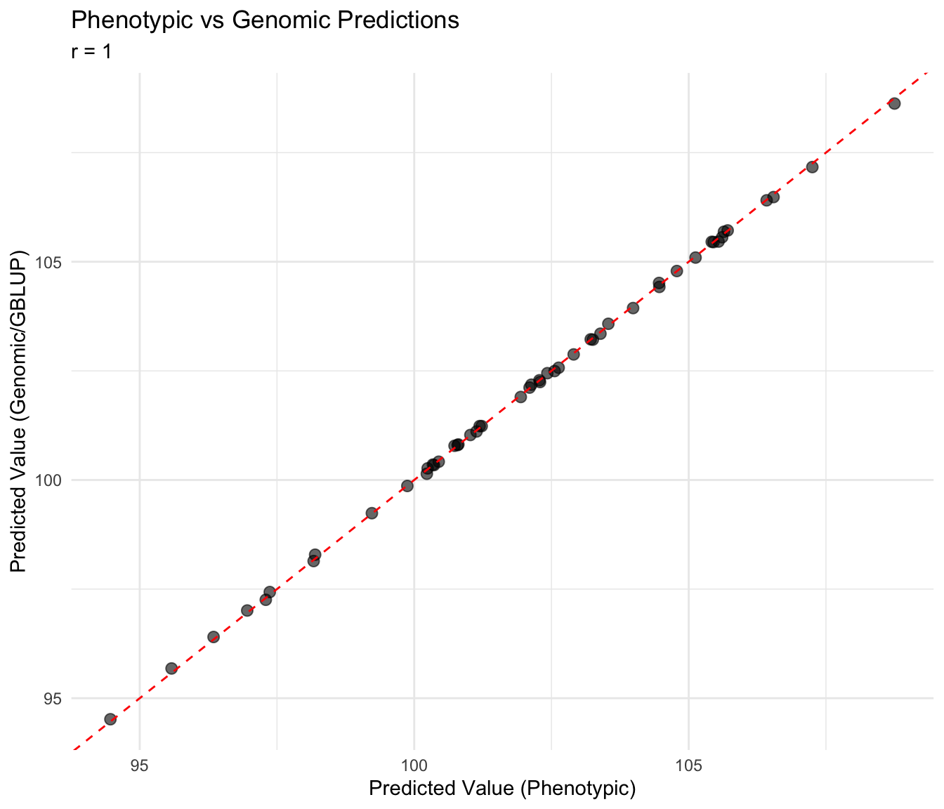

Variance Components Comparison

cat("=== Phenotypic Model Variance Components ===\n")

=== Phenotypic Model Variance Components ===

print(summary(stage2_pheno)$varcomp)

Model statement:
mandala(fixed = yld ~ env, random = ~geno, data = s2_data, matrix_list = list(RMAT = RMAT), 
    R_formula = ~vcov(RMAT))

Variance Components:
 component  estimate std.error  z.ratio bound %ch
      geno 10.202405 2.6120170 3.905949     P  NA
  R.sigma2  3.033944 0.9498473 3.194139     P  NA

Fixed Effects (BLUEs) [first 5]:
      effect   estimate std.error   z.ratio
 (Intercept) 107.191648 0.5145133 208.33601
       envE2 -10.643971 0.3483644 -30.55413
       envE3  -5.506118 0.3483644 -15.80563
       envE4  -4.468908 0.3483644 -12.82826

Converged: TRUE  |  Iterations: 5

Random Effects (BLUPs) [first 5]:
 random level   estimate std.error    z.ratio
   geno  G001  0.5955164 0.9465325  0.6291558
   geno  G002  0.2560207 0.9465325  0.2704828
   geno  G003  3.6784336 0.9465325  3.8862200
   geno  G004 -1.5921461 0.9465325 -1.6820828
   geno  G005  3.5115972 0.9465325  3.7099593

logLik: -528.969   AIC: 1061.937   BIC: 1068.493   logLik_Trunc: -348.857
  component  estimate std.error  z.ratio bound %ch
1      geno 10.202405 2.6120170 3.905949     P  NA
2  R.sigma2  3.033944 0.9498473 3.194139     P  NA

cat("\n=== Genomic Model Variance Components ===\n")

=== Genomic Model Variance Components ===

print(summary(stage2_gblup)$varcomp)

Model statement:
mandala(fixed = yld ~ env, random = ~GM(geno, Gmat), data = s2_data, 
    matrix_list = list(RMAT = RMAT, Gmat = GRM_subset), R_formula = ~vcov(RMAT))

Variance Components:
     component estimate std.error  z.ratio bound %ch
 GM(geno,Gmat) 8.099542 2.0611808 3.929564     P  NA
      R.sigma2 3.121872 0.9564478 3.264028     P  NA

Fixed Effects (BLUEs) [first 5]:
      effect   estimate std.error   z.ratio
 (Intercept) 107.172182 0.2497989 429.03383
       envE2 -10.622852 0.3532820 -30.06904
       envE3  -5.485783 0.3532820 -15.52806
       envE4  -4.448731 0.3532820 -12.59258

Converged: TRUE  |  Iterations: 5

Random Effects (BLUPs) [first 5]:
        random level   estimate std.error    z.ratio
 GM(geno,Gmat)  G001  0.5412109 0.8429880  0.6420149
 GM(geno,Gmat)  G002  0.2130938 0.8409079  0.2534092
 GM(geno,Gmat)  G003  3.6903397 0.8425172  4.3801357
 GM(geno,Gmat)  G004 -1.6155665 0.8429473 -1.9165688
 GM(geno,Gmat)  G005  3.4369444 0.8432061  4.0760431

logLik: -529.382   AIC: 1062.763   BIC: 1069.320   logLik_Trunc: -349.270
      component estimate std.error  z.ratio bound %ch
1 GM(geno,Gmat) 8.099542 2.0611808 3.929564     P  NA
2      R.sigma2 3.121872 0.9564478 3.264028     P  NA

When Does Genomic Prediction Help?

Genomic prediction provides the most benefit when:

Scenario	Benefit
Predicting untested genotypes	GRM allows prediction for genotypes without phenotypic data
Low heritability traits	Genomic info adds signal when phenotypes are noisy
Small family sizes	GRM captures relationships beyond pedigree
Selection accuracy	GEBVs often outperform phenotypic BLUPs

TipCross-Validation

To assess prediction accuracy, use mandala_gp_cv() for cross-validation:

cv_results <- mandala_gp_cv(
  GRM       = GRM,
  data      = s2_data,
  gen_col   = "geno",
  fixed     = yld ~ env,
  random    = ~ GM(geno, Gmat),
  R_formula = ~ vcov(RMAT),
  R_matrix  = RMAT,
  k_folds   = 5,
  n_reps    = 3
)

Summary

TipKey Takeaways

1. GRM integration at Stage 2 enables genomic prediction on BLUEs
2. Use GM(geno, Gmat) to specify genomic relationship structure
3. Combine with vcov(RMAT) to properly weight BLUE uncertainty
4. mandala_grm_prep() handles GRM alignment and scaling
5. mandala_gp() provides a convenient wrapper for the full workflow
6. Genomic predictions are most valuable for untested genotypes and low-heritability traits

Next Steps

• Explore cross-validation with mandala_gp_cv() to assess prediction accuracy
• Consider factor-analytic models (FA()) for complex G×E patterns
• Review the Quick Reference for function details

Session Information

sessionInfo()

R version 4.5.2 (2025-10-31)
Platform: aarch64-apple-darwin20
Running under: macOS Tahoe 26.1

Matrix products: default
BLAS:   /System/Library/Frameworks/Accelerate.framework/Versions/A/Frameworks/vecLib.framework/Versions/A/libBLAS.dylib 
LAPACK: /Library/Frameworks/R.framework/Versions/4.5-arm64/Resources/lib/libRlapack.dylib;  LAPACK version 3.12.1

locale:
[1] C.UTF-8/C.UTF-8/C.UTF-8/C/C.UTF-8/C.UTF-8

time zone: America/New_York
tzcode source: internal

attached base packages:
[1] stats     graphics  grDevices utils     datasets  methods   base     

other attached packages:
[1] Matrix_1.7-4  ggplot2_4.0.0 dplyr_1.1.4   mandala_1.1.0

loaded via a namespace (and not attached):
 [1] vctrs_0.6.5        cli_3.6.5          knitr_1.50         rlang_1.1.6       
 [5] xfun_0.54          generics_0.1.4     S7_0.2.0           splines2_0.5.4    
 [9] jsonlite_2.0.0     labeling_0.4.3     glue_1.8.0         htmltools_0.5.8.1 
[13] scales_1.4.0       rmarkdown_2.30     grid_4.5.2         evaluate_1.0.5    
[17] tibble_3.3.0       fastmap_1.2.0      yaml_2.3.10        lifecycle_1.0.4   
[21] compiler_4.5.2     codetools_0.2-20   RColorBrewer_1.1-3 htmlwidgets_1.6.4 
[25] Rcpp_1.1.0         pkgconfig_2.0.3    farver_2.1.2       lattice_0.22-7    
[29] digest_0.6.37      R6_2.6.1           utf8_1.2.6         tidyselect_1.2.1  
[33] pillar_1.11.1      magrittr_2.0.4     withr_3.0.2        gtable_0.3.6      
[37] tools_4.5.2