Introduction to Mandala

Getting started with agricultural field trial analysis

Overview

The mandala package provides tools for analyzing agricultural field trial data using mixed models. This tutorial introduces the basic concepts and functionality of the package.

What you’ll learn

Installing and loading Mandala
Understanding the key features
Basic model structure for field trials
Running a simple analysis
Visualizing results

Installation

Request the Mandala package download from Listo Agriculture, then install it locally:

# Request a download at https://listoagriculture.com/products

# macOS/Linux (source package)
install.packages("path/to/mandala_x.y.z.tar.gz", repos = NULL, type = "source")

# Windows (binary package)
install.packages("path\\to\\mandala_x.y.z.zip", repos = NULL, type = "win.binary")

Loading Required Packages

# library(mandala)  # Install Mandala first (request download: https://listoagriculture.com/products)
library(dplyr)
library(ggplot2)

Key Features

The mandala package offers:

Mixed Model Analysis — Fit linear mixed models optimized for agricultural field trials
Spatial Analysis — Account for spatial correlation in field layouts
REML/ML Estimation — Flexible estimation methods for variance components
Variance Component Estimation — Extract and interpret genetic and environmental variances
Prediction — Generate BLUPs (Best Linear Unbiased Predictions) and BLUEs

Basic Model Structure

In agricultural field trials, we typically have:

Effect Type	Examples	Purpose
Fixed	Genotypes, treatments	Effects we want to estimate
Random	Blocks, incomplete blocks	Control experimental variation
Spatial	Row, column correlations	Account for field heterogeneity

A typical model might be:

\[ y_{ijk} = \mu + \tau_i + b_j + \epsilon_{ijk} \]

Where:

\(y_{ijk}\) is the observed response (e.g., yield)
\(\mu\) is the overall mean
\(\tau_i\) is the fixed treatment effect (genotype)
\(b_j \sim N(0, \sigma^2_b)\) is the random block effect
\(\epsilon_{ijk} \sim N(0, \sigma^2_e)\) is the residual error

Example: Simple Analysis

Let’s create a simple example dataset to demonstrate the workflow:

# Create example field trial data
set.seed(123)
n_genotypes <- 10
n_blocks <- 4
n_obs <- n_genotypes * n_blocks

example_data <- data.frame(
  genotype = factor(rep(1:n_genotypes, each = n_blocks)),
  block = factor(rep(1:n_blocks, times = n_genotypes)),
  yield = rnorm(n_obs, mean = 100, sd = 10)
)

# Add treatment effects
treatment_effects <- rnorm(n_genotypes, mean = 0, sd = 5)
example_data$yield <- example_data$yield + 
  treatment_effects[as.numeric(example_data$genotype)]

# Add block effects
block_effects <- rnorm(n_blocks, mean = 0, sd = 3)
example_data$yield <- example_data$yield + 
  block_effects[as.numeric(example_data$block)]

head(example_data)

  genotype block     yield
1        1     1  91.68166
2        1     2  94.13905
3        1     3 111.98494
4        1     4 101.33736
5        2     1 101.01325
6        2     2 116.02542

Visualizing the Data

Before fitting any model, it’s important to explore your data:

# Plot yield by genotype
ggplot(example_data, aes(x = genotype, y = yield, color = block)) +
  geom_point(size = 3, alpha = 0.6) +
  theme_minimal() +
  labs(title = "Yield by Genotype and Block",
       x = "Genotype", y = "Yield")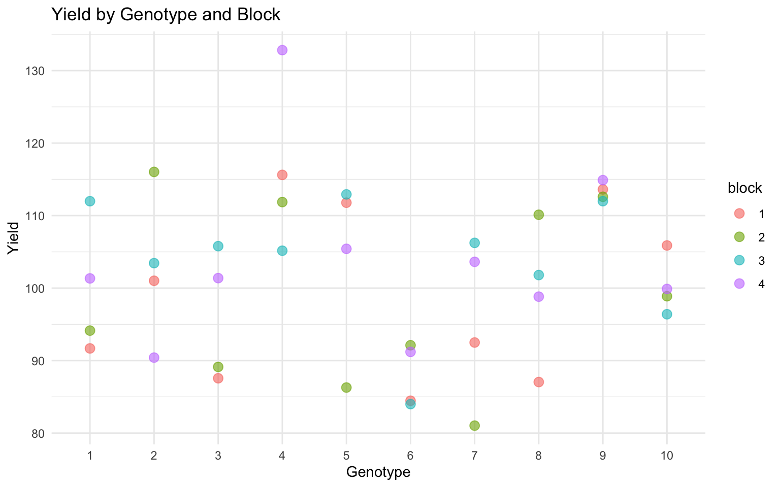

# Summary statistics by genotype
example_data %>%
  group_by(genotype) %>%
  summarise(
    mean_yield = mean(yield),
    sd_yield = sd(yield),
    n = n()
  ) %>%
  head()

# A tibble: 6 × 4
  genotype mean_yield sd_yield     n
  <fct>         <dbl>    <dbl> <int>
1 1              99.8     9.11     4
2 2             103.     10.5      4
3 3              96.0     9.00     4
4 4             116.     11.8      4
5 5             104.     12.3      4
6 6              87.9     4.31     4

Basic Model Fitting

Model Syntax

Mandala uses a clear formula interface:

fixed = yield ~ genotype — fixed effects formula
random = ~ block — random effects formula
data = example_data — your data frame

# Fit a basic mixed model
model <- mandala(
  fixed  = yield ~ genotype,
  random = ~ block,
  data   = example_data
)

# View results
summary(model)

# View variance components
var_comps <- summary(model)$varcomp
print(var_comps)

# Get BLUPs (predicted genotype means)
blups <- mandala_predict(model, classify_term = "genotype")
head(blups)

Model Output Interpretation

When you run summary(model), you’ll typically see:

Variance Components Table
- Genotype variance (σ²_g)
- Block variance (σ²_b)
- Residual variance (σ²_e)
Fixed Effects
- Genotype means (BLUEs)
- Standard errors
Model Fit Statistics
- Log-likelihood
- AIC/BIC

Next Steps

Now that you understand the basics, continue with:

Tutorial 02: Working with Example Datasets — Real-world experimental designs
Tutorial 03: Comparison with Sommer — Quantitative genetics context
Tutorial 04: Comparison with lme4 — General mixed model context

References

Mandala: https://listoagriculture.com/products
Piepho, H.P., et al. (2003). BLUP for phenotypic selection in plant breeding
Best practices for field trial analysis

Session Information

sessionInfo()

R version 4.5.2 (2025-10-31)
Platform: aarch64-apple-darwin20
Running under: macOS Tahoe 26.1

Matrix products: default
BLAS:   /System/Library/Frameworks/Accelerate.framework/Versions/A/Frameworks/vecLib.framework/Versions/A/libBLAS.dylib 
LAPACK: /Library/Frameworks/R.framework/Versions/4.5-arm64/Resources/lib/libRlapack.dylib;  LAPACK version 3.12.1

locale:
[1] en_US.UTF-8/en_US.UTF-8/en_US.UTF-8/C/en_US.UTF-8/en_US.UTF-8

time zone: America/New_York
tzcode source: internal

attached base packages:
[1] stats     graphics  grDevices utils     datasets  methods   base     

other attached packages:
[1] ggplot2_4.0.0 dplyr_1.1.4  

loaded via a namespace (and not attached):
 [1] vctrs_0.6.5        cli_3.6.5          knitr_1.50         rlang_1.1.6       
 [5] xfun_0.54          generics_0.1.4     S7_0.2.0           jsonlite_2.0.0    
 [9] labeling_0.4.3     glue_1.8.0         htmltools_0.5.8.1  scales_1.4.0      
[13] rmarkdown_2.30     grid_4.5.2         evaluate_1.0.5     tibble_3.3.0      
[17] fastmap_1.2.0      yaml_2.3.10        lifecycle_1.0.4    compiler_4.5.2    
[21] RColorBrewer_1.1-3 htmlwidgets_1.6.4  pkgconfig_2.0.3    farver_2.1.2      
[25] digest_0.6.37      R6_2.6.1           utf8_1.2.6         tidyselect_1.2.1  
[29] pillar_1.11.1      magrittr_2.0.4     withr_3.0.2        tools_4.5.2       
[33] gtable_0.3.6