Comparison: Mandala vs Sommer

Side-by-side analysis for quantitative genetics applications

Overview

This tutorial compares the mandala package with the popular sommer package for analyzing agricultural field trials. Both packages are designed for mixed model analysis but have different strengths and use cases.

NoteWhat you’ll learn
  • Key differences between Mandala and Sommer
  • Side-by-side analysis of the same datasets
  • Variance component estimation comparison
  • Heritability calculation methods
  • When to use each package

Background

Sommer Package

  • Purpose: Solving mixed model equations in plant breeding and genetics
  • Key Features:
    • Multivariate models
    • Genomic selection models (GBLUP)
    • AI-REML algorithm
    • Custom relationship matrices
  • Primary Use: Quantitative genetics, genomic prediction

Mandala Package

  • Purpose: Agricultural field trial analysis
  • Key Features:
    • Streamlined workflow for standard designs
    • Built-in spatial analysis (AR1, P-splines)
    • Genomic prediction (GBLUP) with GM() and mandala_gp()
    • Factor-analytic G×E models with FA()
    • User-friendly interface
    • Unified heritability estimation
  • Primary Use: Field trial analysis, variety testing, genomic selection

Loading Packages

library(mandala)
library(sommer)
library(dplyr)
library(ggplot2)
library(tidyr)

Example 1: Simple RCBD

Data Setup

We’ll simulate data with known variance components to validate both approaches:

set.seed(123)
n_genotypes <- 15
n_blocks <- 4

rcbd_data <- expand.grid(
  genotype = factor(paste0("G", sprintf("%02d", 1:n_genotypes))),
  block = factor(paste0("B", 1:n_blocks))
)

# True variance components (for validation)
true_gen_var <- 400
true_block_var <- 100
true_error_var <- 300

# Simulate yield
genotype_effects <- rnorm(n_genotypes, 0, sqrt(true_gen_var))
block_effects <- rnorm(n_blocks, 0, sqrt(true_block_var))

rcbd_data$yield <- 5000 +
  genotype_effects[as.numeric(rcbd_data$genotype)] +
  block_effects[as.numeric(rcbd_data$block)] +
  rnorm(nrow(rcbd_data), 0, sqrt(true_error_var))

head(rcbd_data)
  genotype block    yield
1      G01    B1 4998.471
2      G02    B1 4994.770
3      G03    B1 5045.268
4      G04    B1 5001.508
5      G05    B1 5007.830
6      G06    B1 5041.344
TipTrue Variance Components
  • Genotype variance: 400
  • Block variance: 100
  • Error variance: 300

Analysis with Mandala

#-----------------------------------
# RCBD with Mandala
#-----------------------------------

# Fit model (genotype fixed, block random)
mandala_fixed <- mandala(
  fixed  = yield ~ genotype,
  random = ~ block,
  data   = rcbd_data
)
Initial data rows: 60 
Final data rows after NA handling: 60 
Explicit param_df Check:
      name  type vc_idx     init lower upper origin
1    block   var      1 308.1902 1e-06   Inf      G
2 R.sigma2 R_var      0 385.2378 1e-06   Inf      R
--- Starting EM Warmup ---
EM Warmup: starting theta:
 block 308.2 R.sigma2 385.2 
EM iter 1: logLik=-206.9021; theta: block 232.2 R.sigma2 250.1 
EM iter 2: logLik=-206.5717; theta: block 185.2 R.sigma2 254.4 
EM iter 3: logLik=-206.4858; theta: block 155 R.sigma2 253.6 
EM iter 4 : logLik decreased or failed. Stopping EM.
EM Warmup: ending theta:
 block 155 R.sigma2 253.6 
--- EM Warmup Complete. Starting AI-REML ---
Starting AI-REML logLik = -206.5301
 Iter     LogLik   Sigma2  DF     wall    Restrained
    1  -206.1845   291.327   45  09:48:32  ( 0 restrained)
    2  -206.1845   291.327   45  09:48:32  ( 0 restrained)
Converged at iter 2 by tolerance(s): delta_theta=0.00e+00, delta_loglik=0.00e+00
Main AI-REML Loop finished. Combining results.
solveMME_cpp: adding nugget 1.37303e-08 to MME diagonal (scaled from median diag)
# View variance components
mandala_vc <- summary(mandala_fixed)$varcomp
Model statement:
mandala(fixed = yield ~ genotype, random = ~block, data = rcbd_data)

Variance Components:
 component estimate std.error  z.ratio bound %ch
     block 183.8495 163.95813 1.121320     P  NA
  R.sigma2 291.3273  55.33964 5.264352     P  NA

Fixed Effects (BLUEs) [first 5]:
      effect   estimate std.error     z.ratio
 (Intercept) 4987.83968  10.89921 457.6329403
 genotypeG02   10.87167  12.06907   0.9007884
 genotypeG03   49.15191  12.06907   4.0725532
 genotypeG04   11.44915  12.06907   0.9486360
 genotypeG05   22.73037  12.06907   1.8833577

Converged: TRUE  |  Iterations: 2

Random Effects (BLUPs) [first 5]:
 random level   estimate std.error    z.ratio
  block    B1  11.346109  7.690048  1.4754277
  block    B2   3.995944  7.690048  0.5196254
  block    B3 -18.975978  7.690048 -2.4676021
  block    B4   3.646515  7.690048  0.4741863

logLik: -206.184   AIC: 416.369   BIC: 419.982   logLik_Trunc: -164.832
print(mandala_vc)
  component estimate std.error  z.ratio bound %ch
1     block 183.8495 163.95813 1.121320     P  NA
2  R.sigma2 291.3273  55.33964 5.264352     P  NA
# For heritability: fit genotype as random
mandala_random <- mandala(
  fixed  = yield ~ 1,
  random = ~ genotype + block,
  data   = rcbd_data
)
Initial data rows: 60 
Final data rows after NA handling: 60 
Explicit param_df Check:
      name  type vc_idx     init lower upper origin
1 genotype   var      1 308.1902 1e-06   Inf      G
2    block   var      2 308.1902 1e-06   Inf      G
3 R.sigma2 R_var      0 385.2378 1e-06   Inf      R
--- Starting EM Warmup ---
EM Warmup: starting theta:
 genotype 308.2 block 308.2 R.sigma2 385.2 
EM iter 1: logLik=-270.3482; theta: genotype 261.5 block 232.2 R.sigma2 347.4 
EM iter 2: logLik=-269.9679; theta: genotype 227.8 block 185.2 R.sigma2 384.1 
EM iter 3 : logLik decreased or failed. Stopping EM.
EM Warmup: ending theta:
 genotype 227.8 block 185.2 R.sigma2 384.1 
--- EM Warmup Complete. Starting AI-REML ---
Starting AI-REML logLik = -270.4378
 Iter     LogLik   Sigma2  DF     wall    Restrained
    1  -269.7185   317.436   59  09:48:32  ( 0 restrained)
    2  -269.7185   317.436   59  09:48:32  ( 0 restrained)
Converged at iter 2 by tolerance(s): delta_theta=0.00e+00, delta_loglik=0.00e+00
Main AI-REML Loop finished. Combining results.
solveMME_cpp: adding nugget 1.61414e-08 to MME diagonal (scaled from median diag)
# Unified heritability estimates
h2 <- h2_estimates(
  random_mod = mandala_random,
  fixed_mod  = mandala_fixed,
  genotype   = "genotype"
)
print(h2)
      variable             value
 source_random              TRUE
  source_fixed              TRUE
      sigma_g2  282.451344256933
      sigma_e2  317.435646327182
         n_rep                 4
 mean_PEV_BLUP  76.6522255238933
    avsed_BLUE  12.0691145939918
    vdBLUE_avg  145.663527082907
     H2_Cullis 0.728617947542263
     H2_Piepho 0.795003584626423
       H2_Plot 0.470840922857666
   H2_Standard  0.78066151995103

Note:
Plot and entry mean heritabilities are just the approximation- assuming a single experiment with only 'genotype' and 'error' variance components in the model. For MET, modify the equations and estimate accordingly
# Extract BLUEs
blues <- mandala_fixed$BLUEs
head(blues)
                 effect   estimate std.error     z.ratio
(Intercept) (Intercept) 4987.83968  10.89921 457.6329403
genotypeG02 genotypeG02   10.87167  12.06907   0.9007884
genotypeG03 genotypeG03   49.15191  12.06907   4.0725532
genotypeG04 genotypeG04   11.44915  12.06907   0.9486360
genotypeG05 genotypeG05   22.73037  12.06907   1.8833577
genotypeG06 genotypeG06   52.55270  12.06907   4.3543301

Analysis with Sommer

# Fit model with sommer (genotypes as random for variance estimation)
sommer_model <- mmer(
  fixed = yield ~ 1,
  random = ~ genotype + block,
  data = rcbd_data,
  verbose = FALSE
)

# Extract variance components
sommer_vc <- summary(sommer_model)$varcomp
print("Sommer Variance Components:")
[1] "Sommer Variance Components:"
print(sommer_vc)
                      VarComp VarCompSE   Zratio Constraint
genotype.yield-yield 341.3026 158.12626 2.158418   Positive
block.yield-yield    191.0388 172.26593 1.108976   Positive
units.yield-yield    300.7722  65.65848 4.580858   Positive
# Calculate heritability
var_g <- sommer_vc["genotype", "VarComp"]
var_e <- sommer_vc["units", "VarComp"]
h2_sommer <- var_g / (var_g + var_e / n_blocks)
cat("\nSommer Heritability (entry-mean basis):", round(h2_sommer, 3), "\n")

Sommer Heritability (entry-mean basis): 0.819 
# Extract BLUPs
blups <- randef(sommer_model)$genotype
head(blups)
NULL

Example 2: Multi-Environment Trial

Data Setup

set.seed(456)
n_genotypes <- 20
n_envs <- 3
n_blocks <- 3

met_data <- expand.grid(
  genotype = factor(paste0("G", sprintf("%02d", 1:n_genotypes))),
  env = factor(paste0("E", 1:n_envs)),
  block = factor(paste0("B", 1:n_blocks))
)

# True variance components
true_var_g <- 500
true_var_gxe <- 200
true_var_error <- 400

# Simulate
met_data$yield <- 6000 +
  rnorm(n_genotypes, 0, sqrt(true_var_g))[as.numeric(met_data$genotype)] +
  rnorm(n_envs, 0, 300)[as.numeric(met_data$env)]

# Add GxE
gxe <- matrix(rnorm(n_genotypes * n_envs, 0, sqrt(true_var_gxe)), 
              n_genotypes, n_envs)
met_data$yield <- met_data$yield + 
  gxe[cbind(as.numeric(met_data$genotype), as.numeric(met_data$env))]

# Add block(env) and error
met_data$env_block <- factor(paste0(met_data$env, "_", met_data$block))
met_data$yield <- met_data$yield + 
  rnorm(n_envs * n_blocks, 0, 50)[as.numeric(met_data$env_block)] +
  rnorm(nrow(met_data), 0, sqrt(true_var_error))

head(met_data)
  genotype env block    yield env_block
1      G01  E1    B1 5861.335     E1_B1
2      G02  E1    B1 5902.917     E1_B1
3      G03  E1    B1 5880.556     E1_B1
4      G04  E1    B1 5822.048     E1_B1
5      G05  E1    B1 5856.848     E1_B1
6      G06  E1    B1 5885.062     E1_B1

Sommer MET Analysis

sommer_met <- mmer(
  fixed  = yield ~ env,
  random = ~ genotype + genotype:env + env:block,
  data   = met_data,
  verbose = FALSE
)

# Variance components
met_vc <- summary(sommer_met)$varcomp
print("Sommer MET Variance Components:")
[1] "Sommer MET Variance Components:"
print(met_vc)
                           VarComp VarCompSE   Zratio Constraint
genotype.yield-yield      500.1213 192.74417 2.594742   Positive
genotype:env.yield-yield  127.6429  65.18364 1.958205   Positive
env:block.yield-yield    1347.2640 790.20255 1.704960   Positive
units.yield-yield         432.1280  57.23833 7.549626   Positive
# Extract components
var_g <- met_vc["genotype", "VarComp"]
var_gxe <- met_vc["genotype:env", "VarComp"]
var_e <- met_vc["units", "VarComp"]

# Entry-mean heritability across environments
h2_met <- var_g / (var_g + var_gxe/n_envs + var_e/(n_envs * n_blocks))
cat("\nEntry-mean heritability:", round(h2_met, 3), "\n")

Entry-mean heritability: NA 

Example 3: Spatial Analysis

set.seed(789)
n_rows <- 10
n_cols <- 10

spatial_data <- data.frame(
  row = rep(1:n_rows, each = n_cols),
  col = rep(1:n_cols, times = n_rows),
  genotype = factor(sample(paste0("G", 1:25), n_rows * n_cols, replace = TRUE))
)

# Add spatial trend + genotype effects + error
gen_eff <- setNames(rnorm(25, 0, 300), paste0("G", 1:25))
spatial_data$yield <- 5000 + 
  gen_eff[spatial_data$genotype] +
  30 * spatial_data$row - 20 * spatial_data$col +
  rnorm(nrow(spatial_data), 0, 200)

Visualize Field Pattern

ggplot(spatial_data, aes(x = col, y = row, fill = yield)) +
  geom_tile() +
  scale_fill_gradient2(low = "#2E6B8A", mid = "#FAF8F5", high = "#9B5B5B",
                       midpoint = mean(spatial_data$yield)) +
  coord_equal() +
  theme_minimal() +
  labs(title = "Field Map - Spatial Trend Visible",
       x = "Column", y = "Row")

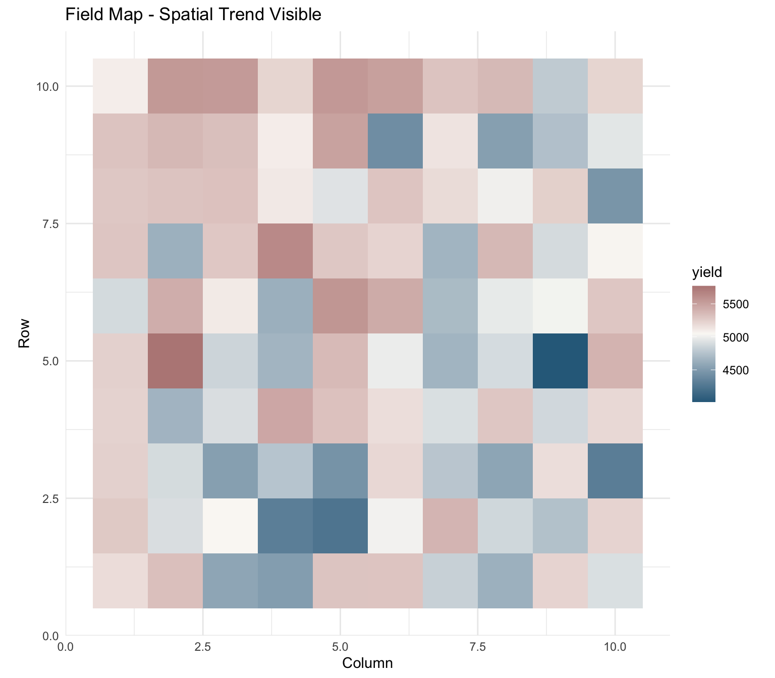
Sommer with Row-Column Effects

spatial_data$row_f <- factor(spatial_data$row)
spatial_data$col_f <- factor(spatial_data$col)

sommer_spatial <- mmer(
  fixed = yield ~ 1,
  random = ~ genotype + row_f + col_f,
  data = spatial_data,
  verbose = FALSE
)

print(summary(sommer_spatial)$varcomp)
                        VarComp VarCompSE    Zratio Constraint
genotype.yield-yield 62242.1591 22296.159 2.7916091   Positive
row_f.yield-yield    11391.4155  8201.081 1.3890139   Positive
col_f.yield-yield      490.7583  3227.847 0.1520389   Positive
units.yield-yield    47209.7972  8710.007 5.4201793   Positive

Example 4: Genomic Prediction (GBLUP)

Both packages now support GBLUP with relationship matrices. Here’s how they compare:

Sommer GBLUP

# Create a simple kinship matrix (in practice, use marker data)
library(sommer)

# Simulated GRM
set.seed(123)
n_geno <- 50
G <- matrix(rnorm(n_geno * n_geno), n_geno, n_geno)
G <- G %*% t(G) / ncol(G)
rownames(G) <- colnames(G) <- paste0("G", 1:n_geno)

# Phenotype data
gblup_data <- data.frame(
  geno = factor(paste0("G", 1:n_geno)),
  yield = rnorm(n_geno, 5000, 300)
)

# Sommer GBLUP
sommer_gblup <- mmer(
  fixed = yield ~ 1,
  random = ~ vsr(geno, Gu = G),
  data = gblup_data,
  verbose = FALSE
)

# Extract GEBVs
gebvs_sommer <- randef(sommer_gblup)$`u:geno`

Mandala GBLUP

# Prepare GRM for Mandala
grm_prep <- mandala_grm_prep(
  GRM       = G,
  data      = gblup_data,
  gen_col   = "geno",
  GRM_label = "GRM"
)

# Mandala GBLUP
mandala_gblup <- mandala(
  fixed       = yield ~ 1,
  random      = ~ GM(geno, GRM),
  matrix_list = grm_prep,
  data        = gblup_data
)
Initial data rows: 50 
Final data rows after NA handling: 50 
Explicit param_df Check:
          name  type vc_idx     init lower upper origin
1 GM(geno,GRM)   var      1 37618.02 1e-06   Inf      G
2     R.sigma2 R_var      0 47022.53 1e-06   Inf      R
--- Starting EM Warmup ---
EM Warmup: starting theta:
 GM(geno,GRM) 37620 R.sigma2 47020 
EM iter 1: logLik=-352.1874; theta: GM(geno,GRM) 6313000 R.sigma2 35430 
EM iter 2 : logLik decreased or failed. Stopping EM.
EM Warmup: ending theta:
 GM(geno,GRM) 6313000 R.sigma2 35430 
--- EM Warmup Complete. Starting AI-REML ---
Starting AI-REML logLik = -431.1061
 Iter     LogLik   Sigma2  DF     wall    Restrained
    1  -424.5816 43930.846   49  09:48:32  ( 0 restrained)
    2  -418.1446 54474.249   49  09:48:32  ( 0 restrained)
    3  -414.7927 115851.644   49  09:48:32  ( 0 restrained)
    4  -411.5665 172076.869   49  09:48:32  ( 0 restrained)
    5  -408.2658 201201.708   49  09:48:32  ( 0 restrained)
    6  -404.8119 203297.545   49  09:48:32  ( 0 restrained)
    7  -401.2479 190208.821   49  09:48:32  ( 0 restrained)
    8  -397.6812 174435.200   49  09:48:32  ( 0 restrained)
    9  -394.2170 163116.078   49  09:48:32  ( 0 restrained)
   10  -390.9134 157581.971   49  09:48:32  ( 0 restrained)
   11  -387.7733 155733.717   49  09:48:32  ( 0 restrained)
   12  -384.7654 154764.440   49  09:48:32  ( 0 restrained)
   13  -381.8571 152867.446   49  09:48:32  ( 0 restrained)
   14  -379.0363 149626.751   49  09:48:32  ( 0 restrained)
   15  -376.3150 145530.523   49  09:48:32  ( 0 restrained)
   16  -373.7185 141280.347   49  09:48:32  ( 0 restrained)
   17  -371.2714 137343.664   49  09:48:32  ( 0 restrained)
   18  -368.9886 133847.494   49  09:48:32  ( 0 restrained)
   19  -366.8745 130692.229   49  09:48:32  ( 0 restrained)
   20  -364.9270 127718.127   49  09:48:32  ( 0 restrained)
   21  -363.1426 124815.885   49  09:48:32  ( 0 restrained)
   22  -361.5192 121955.051   49  09:48:32  ( 0 restrained)
   23  -360.0554 119158.283   49  09:48:32  ( 0 restrained)
   24  -358.7496 116462.230   49  09:48:32  ( 0 restrained)
   25  -357.5974 113891.550   49  09:48:32  ( 0 restrained)
   26  -356.5918 111452.250   49  09:48:32  ( 0 restrained)
   27  -355.7234 109137.707   49  09:48:32  ( 0 restrained)
   28  -354.9814 106937.854   49  09:48:32  ( 0 restrained)
   29  -354.3544 104845.395   49  09:48:32  ( 0 restrained)
   30  -353.8310 102857.563   49  09:48:32  ( 0 restrained)
   31  -353.3999 100974.888   49  09:48:32  ( 0 restrained)
   32  -353.0502 99199.106   49  09:48:32  ( 0 restrained)
   33  -352.7712 97531.616   49  09:48:32  ( 0 restrained)
   34  -352.5529 95972.857   49  09:48:32  ( 0 restrained)
   35  -352.3860 94522.328   49  09:48:32  ( 0 restrained)
   36  -352.2619 93178.825   49  09:48:32  ( 0 restrained)
   37  -352.1729 91940.594   49  09:48:32  ( 0 restrained)
   38  -352.1124 90805.333   49  09:48:32  ( 0 restrained)
   39  -352.0745 89770.117   49  09:48:32  ( 0 restrained)
   40  -352.0540 88831.325   49  09:48:32  ( 0 restrained)
   41  -352.0476 87984.630   49  09:48:32  ( 0 restrained)
   42  -352.0465 87373.428   49  09:48:32  ( 0 restrained)
   43  -352.0465 87373.428   49  09:48:32  ( 0 restrained)
Converged at iter 43 by tolerance(s): delta_theta=0.00e+00, delta_loglik=0.00e+00
Main AI-REML Loop finished. Combining results.
solveMME_cpp: adding nugget 3.46386e-08 to MME diagonal (scaled from median diag)
# Extract predictions
gebvs_mandala <- mandala_predict(mandala_gblup, classify_term = "geno")

Notes:
- The predictions are obtained by averaging across the hypertable
  calculated from model terms constructed solely from factors in
  the averaging and classify sets.
- The simple averaging set: (none)
# Or use the high-level wrapper with cross-validation
cv_results <- mandala_gp_cv(
  fixed     = yield ~ 1,
  random    = ~ GM(geno, GRM),
  gen_col   = "geno",
  data      = gblup_data,
  GRM       = G,
  k_folds   = 5,
  n_reps    = 3
)
Initial data rows: 40 
Final data rows after NA handling: 40 
Explicit param_df Check:
          name  type vc_idx     init lower upper origin
1 GM(geno,GRM)   var      1 35789.19 1e-06   Inf      G
2     R.sigma2 R_var      0 44736.49 1e-06   Inf      R
--- Starting EM Warmup ---
EM Warmup: starting theta:
 GM(geno,GRM) 35790 R.sigma2 44740 
EM iter 1: logLik=-279.6282; theta: GM(geno,GRM) 126600 R.sigma2 27130 
EM iter 2 : logLik decreased or failed. Stopping EM.
EM Warmup: ending theta:
 GM(geno,GRM) 126600 R.sigma2 27130 
--- EM Warmup Complete. Starting AI-REML ---
Starting AI-REML logLik = -281.9186
 Iter     LogLik   Sigma2  DF     wall    Restrained
    1  -280.7147 33646.834   39  09:48:32  ( 0 restrained)
    2  -280.0755 41722.074   39  09:48:32  ( 0 restrained)
    3  -280.0755 41722.074   39  09:48:32  ( 0 restrained)
Converged at iter 3 by tolerance(s): delta_theta=0.00e+00, delta_loglik=0.00e+00
Main AI-REML Loop finished. Combining results.
solveMME_cpp: adding nugget 1.002e-10 to MME diagonal (scaled from median diag)
Initial data rows: 40 
Final data rows after NA handling: 40 
Explicit param_df Check:
          name  type vc_idx     init lower upper origin
1 GM(geno,GRM)   var      1 33453.99 1e-06   Inf      G
2     R.sigma2 R_var      0 41817.49 1e-06   Inf      R
--- Starting EM Warmup ---
EM Warmup: starting theta:
 GM(geno,GRM) 33450 R.sigma2 41820 
EM iter 1: logLik=-278.3124; theta: GM(geno,GRM) 158300 R.sigma2 20390 
EM iter 2 : logLik decreased or failed. Stopping EM.
EM Warmup: ending theta:
 GM(geno,GRM) 158300 R.sigma2 20390 
--- EM Warmup Complete. Starting AI-REML ---
Starting AI-REML logLik = -282.6316
 Iter     LogLik   Sigma2  DF     wall    Restrained
    1  -280.7119 25284.008   39  09:48:33  ( 0 restrained)
    2  -279.4704 31352.170   39  09:48:33  ( 0 restrained)
    3  -279.4704 31352.170   39  09:48:33  ( 0 restrained)
Converged at iter 3 by tolerance(s): delta_theta=0.00e+00, delta_loglik=0.00e+00
Main AI-REML Loop finished. Combining results.
solveMME_cpp: adding nugget 7.63712e-11 to MME diagonal (scaled from median diag)
Initial data rows: 40 
Final data rows after NA handling: 40 
Explicit param_df Check:
          name  type vc_idx     init lower upper origin
1 GM(geno,GRM)   var      1 40092.12 1e-06   Inf      G
2     R.sigma2 R_var      0 50115.15 1e-06   Inf      R
--- Starting EM Warmup ---
EM Warmup: starting theta:
 GM(geno,GRM) 40090 R.sigma2 50120 
EM iter 1: logLik=-281.8421; theta: GM(geno,GRM) 296900 R.sigma2 31180 
EM iter 2 : logLik decreased or failed. Stopping EM.
EM Warmup: ending theta:
 GM(geno,GRM) 296900 R.sigma2 31180 
--- EM Warmup Complete. Starting AI-REML ---
Starting AI-REML logLik = -291.3121
 Iter     LogLik   Sigma2  DF     wall    Restrained
    1  -288.5344 38662.955   39  09:48:33  ( 0 restrained)
    2  -286.4180 47942.064   39  09:48:33  ( 0 restrained)
    3  -286.4180 47942.064   39  09:48:33  ( 0 restrained)
Converged at iter 3 by tolerance(s): delta_theta=0.00e+00, delta_loglik=0.00e+00
Main AI-REML Loop finished. Combining results.
solveMME_cpp: adding nugget 5.60422e-11 to MME diagonal (scaled from median diag)
Initial data rows: 40 
Final data rows after NA handling: 40 
Explicit param_df Check:
          name  type vc_idx     init lower upper origin
1 GM(geno,GRM)   var      1 39877.09 1e-06   Inf      G
2     R.sigma2 R_var      0 49846.37 1e-06   Inf      R
--- Starting EM Warmup ---
EM Warmup: starting theta:
 GM(geno,GRM) 39880 R.sigma2 49850 
EM iter 1: logLik=-281.7372; theta: GM(geno,GRM) 150300 R.sigma2 24310 
EM iter 2 : logLik decreased or failed. Stopping EM.
EM Warmup: ending theta:
 GM(geno,GRM) 150300 R.sigma2 24310 
--- EM Warmup Complete. Starting AI-REML ---
Starting AI-REML logLik = -284.1892
 Iter     LogLik   Sigma2  DF     wall    Restrained
    1  -282.8124 30146.779   39  09:48:33  ( 0 restrained)
    2  -282.0639 37382.006   39  09:48:33  ( 0 restrained)
    3  -282.0639 37382.006   39  09:48:33  ( 0 restrained)
Converged at iter 3 by tolerance(s): delta_theta=0.00e+00, delta_loglik=0.00e+00
Main AI-REML Loop finished. Combining results.
solveMME_cpp: adding nugget 7.581e-11 to MME diagonal (scaled from median diag)
Initial data rows: 40 
Final data rows after NA handling: 40 
Explicit param_df Check:
          name  type vc_idx     init lower upper origin
1 GM(geno,GRM)   var      1 38476.74 1e-06   Inf      G
2     R.sigma2 R_var      0 48095.92 1e-06   Inf      R
--- Starting EM Warmup ---
EM Warmup: starting theta:
 GM(geno,GRM) 38480 R.sigma2 48100 
EM iter 1: logLik=-281.0401; theta: GM(geno,GRM) 114800 R.sigma2 23480 
EM iter 2 : logLik decreased or failed. Stopping EM.
EM Warmup: ending theta:
 GM(geno,GRM) 114800 R.sigma2 23480 
--- EM Warmup Complete. Starting AI-REML ---
Starting AI-REML logLik = -282.0713
 Iter     LogLik   Sigma2  DF     wall    Restrained
    1  -281.2607 29119.621   39  09:48:33  ( 0 restrained)
    2  -280.9657 36108.330   39  09:48:33  ( 0 restrained)
    3  -280.9657 36108.330   39  09:48:33  ( 0 restrained)
Converged at iter 3 by tolerance(s): delta_theta=0.00e+00, delta_loglik=0.00e+00
Main AI-REML Loop finished. Combining results.
solveMME_cpp: adding nugget 9.42742e-11 to MME diagonal (scaled from median diag)
Initial data rows: 40 
Final data rows after NA handling: 40 
Explicit param_df Check:
          name  type vc_idx     init lower upper origin
1 GM(geno,GRM)   var      1 42247.50 1e-06   Inf      G
2     R.sigma2 R_var      0 52809.37 1e-06   Inf      R
--- Starting EM Warmup ---
EM Warmup: starting theta:
 GM(geno,GRM) 42250 R.sigma2 52810 
EM iter 1: logLik=-282.8632; theta: GM(geno,GRM) 227200 R.sigma2 29380 
EM iter 2 : logLik decreased or failed. Stopping EM.
EM Warmup: ending theta:
 GM(geno,GRM) 227200 R.sigma2 29380 
--- EM Warmup Complete. Starting AI-REML ---
Starting AI-REML logLik = -288.5851
 Iter     LogLik   Sigma2  DF     wall    Restrained
    1  -286.4180 36431.416   39  09:48:33  ( 0 restrained)
    2  -284.9281 45174.956   39  09:48:33  ( 0 restrained)
    3  -284.9281 45174.956   39  09:48:33  ( 0 restrained)
Converged at iter 3 by tolerance(s): delta_theta=0.00e+00, delta_loglik=0.00e+00
Main AI-REML Loop finished. Combining results.
solveMME_cpp: adding nugget 5.78483e-11 to MME diagonal (scaled from median diag)
Initial data rows: 40 
Final data rows after NA handling: 40 
Explicit param_df Check:
          name  type vc_idx     init lower upper origin
1 GM(geno,GRM)   var      1 40784.60 1e-06   Inf      G
2     R.sigma2 R_var      0 50980.75 1e-06   Inf      R
--- Starting EM Warmup ---
EM Warmup: starting theta:
 GM(geno,GRM) 40780 R.sigma2 50980 
EM iter 1: logLik=-282.1760; theta: GM(geno,GRM) 262600 R.sigma2 24950 
EM iter 2 : logLik decreased or failed. Stopping EM.
EM Warmup: ending theta:
 GM(geno,GRM) 262600 R.sigma2 24950 
--- EM Warmup Complete. Starting AI-REML ---
Starting AI-REML logLik = -289.6977
 Iter     LogLik   Sigma2  DF     wall    Restrained
    1  -287.0971 30940.835   39  09:48:33  ( 0 restrained)
    2  -285.1689 38366.636   39  09:48:33  ( 0 restrained)
    3  -285.1689 38366.636   39  09:48:33  ( 0 restrained)
Converged at iter 3 by tolerance(s): delta_theta=0.00e+00, delta_loglik=0.00e+00
Main AI-REML Loop finished. Combining results.
solveMME_cpp: adding nugget 5.4516e-11 to MME diagonal (scaled from median diag)
Initial data rows: 40 
Final data rows after NA handling: 40 
Explicit param_df Check:
          name  type vc_idx     init lower upper origin
1 GM(geno,GRM)   var      1 32118.43 1e-06   Inf      G
2     R.sigma2 R_var      0 40148.04 1e-06   Inf      R
--- Starting EM Warmup ---
EM Warmup: starting theta:
 GM(geno,GRM) 32120 R.sigma2 40150 
EM iter 1: logLik=-277.5180; theta: GM(geno,GRM) 84860 R.sigma2 21350 
EM iter 2 : logLik decreased or failed. Stopping EM.
EM Warmup: ending theta:
 GM(geno,GRM) 84860 R.sigma2 21350 
--- EM Warmup Complete. Starting AI-REML ---
Starting AI-REML logLik = -278.1024
 Iter     LogLik   Sigma2  DF     wall    Restrained
    1  -277.5516 26474.746   39  09:48:33  ( 0 restrained)
    2  -277.4094 32828.686   39  09:48:33  ( 0 restrained)
    3  -277.4094 32828.686   39  09:48:33  ( 0 restrained)
Converged at iter 3 by tolerance(s): delta_theta=0.00e+00, delta_loglik=0.00e+00
Main AI-REML Loop finished. Combining results.
solveMME_cpp: adding nugget 1.14443e-10 to MME diagonal (scaled from median diag)
Initial data rows: 40 
Final data rows after NA handling: 40 
Explicit param_df Check:
          name  type vc_idx     init lower upper origin
1 GM(geno,GRM)   var      1 35369.82 1e-06   Inf      G
2     R.sigma2 R_var      0 44212.28 1e-06   Inf      R
--- Starting EM Warmup ---
EM Warmup: starting theta:
 GM(geno,GRM) 35370 R.sigma2 44210 
EM iter 1: logLik=-279.3983; theta: GM(geno,GRM) 98200 R.sigma2 21580 
EM iter 2 : logLik decreased or failed. Stopping EM.
EM Warmup: ending theta:
 GM(geno,GRM) 98200 R.sigma2 21580 
--- EM Warmup Complete. Starting AI-REML ---
Starting AI-REML logLik = -280.0997
 Iter     LogLik   Sigma2  DF     wall    Restrained
    1  -279.4606 26754.880   39  09:48:33  ( 0 restrained)
    2  -279.2888 33176.051   39  09:48:33  ( 0 restrained)
    3  -279.2888 33176.051   39  09:48:33  ( 0 restrained)
Converged at iter 3 by tolerance(s): delta_theta=0.00e+00, delta_loglik=0.00e+00
Main AI-REML Loop finished. Combining results.
solveMME_cpp: adding nugget 1.27447e-10 to MME diagonal (scaled from median diag)
Initial data rows: 40 
Final data rows after NA handling: 40 
Explicit param_df Check:
          name  type vc_idx     init lower upper origin
1 GM(geno,GRM)   var      1 36765.32 1e-06   Inf      G
2     R.sigma2 R_var      0 45956.64 1e-06   Inf      R
--- Starting EM Warmup ---
EM Warmup: starting theta:
 GM(geno,GRM) 36770 R.sigma2 45960 
EM iter 1: logLik=-280.1529; theta: GM(geno,GRM) 199000 R.sigma2 23750 
EM iter 2 : logLik decreased or failed. Stopping EM.
EM Warmup: ending theta:
 GM(geno,GRM) 199000 R.sigma2 23750 
--- EM Warmup Complete. Starting AI-REML ---
Starting AI-REML logLik = -285.8463
 Iter     LogLik   Sigma2  DF     wall    Restrained
    1  -283.6389 29444.262   39  09:48:33  ( 0 restrained)
    2  -282.1126 36510.884   39  09:48:33  ( 0 restrained)
    3  -282.1126 36510.884   39  09:48:33  ( 0 restrained)
Converged at iter 3 by tolerance(s): delta_theta=0.00e+00, delta_loglik=0.00e+00
Main AI-REML Loop finished. Combining results.
solveMME_cpp: adding nugget 6.89168e-11 to MME diagonal (scaled from median diag)
Initial data rows: 40 
Final data rows after NA handling: 40 
Explicit param_df Check:
          name  type vc_idx     init lower upper origin
1 GM(geno,GRM)   var      1 38482.06 1e-06   Inf      G
2     R.sigma2 R_var      0 48102.58 1e-06   Inf      R
--- Starting EM Warmup ---
EM Warmup: starting theta:
 GM(geno,GRM) 38480 R.sigma2 48100 
EM iter 1: logLik=-281.0428; theta: GM(geno,GRM) 182900 R.sigma2 23530 
EM iter 2 : logLik decreased or failed. Stopping EM.
EM Warmup: ending theta:
 GM(geno,GRM) 182900 R.sigma2 23530 
--- EM Warmup Complete. Starting AI-REML ---
Starting AI-REML logLik = -285.4055
 Iter     LogLik   Sigma2  DF     wall    Restrained
    1  -283.4766 29177.766   39  09:48:33  ( 0 restrained)
    2  -282.2259 36180.430   39  09:48:33  ( 0 restrained)
    3  -282.2259 36180.430   39  09:48:33  ( 0 restrained)
Converged at iter 3 by tolerance(s): delta_theta=0.00e+00, delta_loglik=0.00e+00
Main AI-REML Loop finished. Combining results.
solveMME_cpp: adding nugget 7.45502e-11 to MME diagonal (scaled from median diag)
Initial data rows: 40 
Final data rows after NA handling: 40 
Explicit param_df Check:
          name  type vc_idx     init lower upper origin
1 GM(geno,GRM)   var      1 38594.76 1e-06   Inf      G
2     R.sigma2 R_var      0 48243.44 1e-06   Inf      R
--- Starting EM Warmup ---
EM Warmup: starting theta:
 GM(geno,GRM) 38590 R.sigma2 48240 
EM iter 1: logLik=-281.0998; theta: GM(geno,GRM) 241200 R.sigma2 35600 
EM iter 2 : logLik decreased or failed. Stopping EM.
EM Warmup: ending theta:
 GM(geno,GRM) 241200 R.sigma2 35600 
--- EM Warmup Complete. Starting AI-REML ---
Starting AI-REML logLik = -288.8364
 Iter     LogLik   Sigma2  DF     wall    Restrained
    1  -286.4824 44148.552   39  09:48:33  ( 0 restrained)
    2  -284.8093 54744.204   39  09:48:33  ( 0 restrained)
    3  -284.8093 54744.204   39  09:48:33  ( 0 restrained)
Converged at iter 3 by tolerance(s): delta_theta=0.00e+00, delta_loglik=0.00e+00
Main AI-REML Loop finished. Combining results.
solveMME_cpp: adding nugget 4.82012e-11 to MME diagonal (scaled from median diag)
Initial data rows: 40 
Final data rows after NA handling: 40 
Explicit param_df Check:
          name  type vc_idx     init lower upper origin
1 GM(geno,GRM)   var      1 32967.04 1e-06   Inf      G
2     R.sigma2 R_var      0 41208.81 1e-06   Inf      R
--- Starting EM Warmup ---
EM Warmup: starting theta:
 GM(geno,GRM) 32970 R.sigma2 41210 
EM iter 1: logLik=-278.0265; theta: GM(geno,GRM) 130300 R.sigma2 21210 
EM iter 2 : logLik decreased or failed. Stopping EM.
EM Warmup: ending theta:
 GM(geno,GRM) 130300 R.sigma2 21210 
--- EM Warmup Complete. Starting AI-REML ---
Starting AI-REML logLik = -280.8927
 Iter     LogLik   Sigma2  DF     wall    Restrained
    1  -279.4098 26302.210   39  09:48:33  ( 0 restrained)
    2  -278.5607 32614.741   39  09:48:33  ( 0 restrained)
    3  -278.5607 32614.741   39  09:48:33  ( 0 restrained)
Converged at iter 3 by tolerance(s): delta_theta=0.00e+00, delta_loglik=0.00e+00
Main AI-REML Loop finished. Combining results.
solveMME_cpp: adding nugget 9.50786e-11 to MME diagonal (scaled from median diag)
Initial data rows: 40 
Final data rows after NA handling: 40 
Explicit param_df Check:
          name  type vc_idx     init lower upper origin
1 GM(geno,GRM)   var      1 35026.28 1e-06   Inf      G
2     R.sigma2 R_var      0 43782.85 1e-06   Inf      R
--- Starting EM Warmup ---
EM Warmup: starting theta:
 GM(geno,GRM) 35030 R.sigma2 43780 
EM iter 1: logLik=-279.2080; theta: GM(geno,GRM) 116300 R.sigma2 22640 
EM iter 2 : logLik decreased or failed. Stopping EM.
EM Warmup: ending theta:
 GM(geno,GRM) 116300 R.sigma2 22640 
--- EM Warmup Complete. Starting AI-REML ---
Starting AI-REML logLik = -280.8900
 Iter     LogLik   Sigma2  DF     wall    Restrained
    1  -279.8198 28072.906   39  09:48:33  ( 0 restrained)
    2  -279.3120 34810.404   39  09:48:33  ( 0 restrained)
    3  -279.3120 34810.404   39  09:48:33  ( 0 restrained)
Converged at iter 3 by tolerance(s): delta_theta=0.00e+00, delta_loglik=0.00e+00
Main AI-REML Loop finished. Combining results.
solveMME_cpp: adding nugget 9.04255e-11 to MME diagonal (scaled from median diag)
Initial data rows: 40 
Final data rows after NA handling: 40 
Explicit param_df Check:
          name  type vc_idx     init lower upper origin
1 GM(geno,GRM)   var      1 43744.72 1e-06   Inf      G
2     R.sigma2 R_var      0 54680.90 1e-06   Inf      R
--- Starting EM Warmup ---
EM Warmup: starting theta:
 GM(geno,GRM) 43740 R.sigma2 54680 
EM iter 1: logLik=-283.5423; theta: GM(geno,GRM) 184500 R.sigma2 34000 
EM iter 2 : logLik decreased or failed. Stopping EM.
EM Warmup: ending theta:
 GM(geno,GRM) 184500 R.sigma2 34000 
--- EM Warmup Complete. Starting AI-REML ---
Starting AI-REML logLik = -287.1877
 Iter     LogLik   Sigma2  DF     wall    Restrained
    1  -285.5968 42160.162   39  09:48:33  ( 0 restrained)
    2  -284.6348 52278.601   39  09:48:33  ( 0 restrained)
    3  -284.6348 52278.601   39  09:48:33  ( 0 restrained)
Converged at iter 3 by tolerance(s): delta_theta=0.00e+00, delta_loglik=0.00e+00
Main AI-REML Loop finished. Combining results.
solveMME_cpp: adding nugget 5.69856e-11 to MME diagonal (scaled from median diag)
mean(cv_results$by_fold$pred_ability)
[1] -0.06676604

Example 5: Factor-Analytic G×E Models

For complex multi-environment trials, both packages support factor-analytic variance structures:

Sommer FA Model

# Sommer uses dsr() for diagonal structures
# FA models require more manual setup
sommer_diag <- mmer(
  fixed = yield ~ env,
  random = ~ vsr(dsr(env), geno),  # Diagonal G×E
  data = met_data,
  verbose = FALSE
)

Mandala FA Model

# Mandala provides dedicated FA() syntax
fa_model <- mandala(
  fixed  = yield ~ env + geno,
  random = ~ FA(geno, env, k = 2) + by(env):ar1(row) + by(env):ar1(col),
  data   = met_data
)
Initial data rows: 180 
Final data rows after NA handling: 180 
Explicit param_df Check:
               name      type vc_idx      init    lower upper origin value
1   FA_lambda_E1_F1 fa_lambda      1     0.100  1.0e+00  1.00      G     1
2   FA_lambda_E2_F1 fa_lambda      1     0.100     -Inf   Inf      G     1
3   FA_lambda_E3_F1 fa_lambda      1     0.100     -Inf   Inf      G     1
4   FA_lambda_E2_F2 fa_lambda      1     0.100     -Inf   Inf      G     1
5   FA_lambda_E3_F2 fa_lambda      1     0.100     -Inf   Inf      G     1
6         FA_psi_E1    fa_psi      1  4437.864  1.0e-06   Inf      G     1
7         FA_psi_E2    fa_psi      1  4437.864  1.0e-06   Inf      G     1
8         FA_psi_E3    fa_psi      1  4437.864  1.0e-06   Inf      G     1
9      FA(geno:env)       var      1 13313.591  1.0e-06   Inf      G     1
10 at(env):ar1(row)       var      2 13313.591  1.0e-06   Inf      G     1
11   rho_by.env.row    rho_by      2     0.500 -9.5e-01  0.95      G     1
12 at(env):ar1(col)       var      3 13313.591  1.0e-06   Inf      G     1
13   rho_by.env.col    rho_by      3     0.500 -9.5e-01  0.95      G     1
14         R.sigma2     R_var      0 16641.988  1.0e-06   Inf      R    NA
--- EM Warmup Skipped. Starting AI-REML ---
Starting AI-REML logLik = -979.5626
 Iter     LogLik   Sigma2  DF     wall    Restrained
    1  -972.9567 14940.790  158  09:48:33  ( 4 restrained)
    2  -964.7759 13054.135  158  09:48:33  ( 4 restrained)
 Froze FA_lambda_E1_F1 at 1.000000e-05
 Froze FA_lambda_E2_F1 at 1.000000e-05
 Froze FA_lambda_E3_F1 at 1.000000e-05
 Froze FA_lambda_E2_F2 at 9.999469e-06
 Froze FA_lambda_E3_F2 at 9.999464e-06
 Froze FA(geno:env) at 1.000000e-05
    3  -959.7265 11996.704  158  09:48:34  ( 8 restrained)
    4  -952.3940 10589.926  158  09:48:34  ( 8 restrained)
    5  -943.8895  9140.642  158  09:48:34  ( 8 restrained)
    6  -933.7639  7642.500  158  09:48:34  ( 8 restrained)
    7  -921.4768  6111.802  158  09:48:34  ( 8 restrained)
    8  -906.2974  4583.027  158  09:48:34  ( 8 restrained)
    9  -887.4193  3121.805  158  09:48:34  ( 8 restrained)
   10  -864.8827  1836.025  158  09:48:34  ( 8 restrained)
   11  -844.8995   864.658  158  09:48:34  ( 8 restrained)
   12  -843.8324   594.878  158  09:48:34  ( 8 restrained)
   13  -843.8324   594.878  158  09:48:35  ( 8 restrained)
Converged at iter 13 by tolerance(s): delta_theta=0.00e+00, delta_loglik=0.00e+00
Main AI-REML Loop finished. Combining results.
solveMME_cpp: adding nugget 1.0964e-08 to MME diagonal (scaled from median diag)
# Built-in visualization
fa_biplot(fa_model)

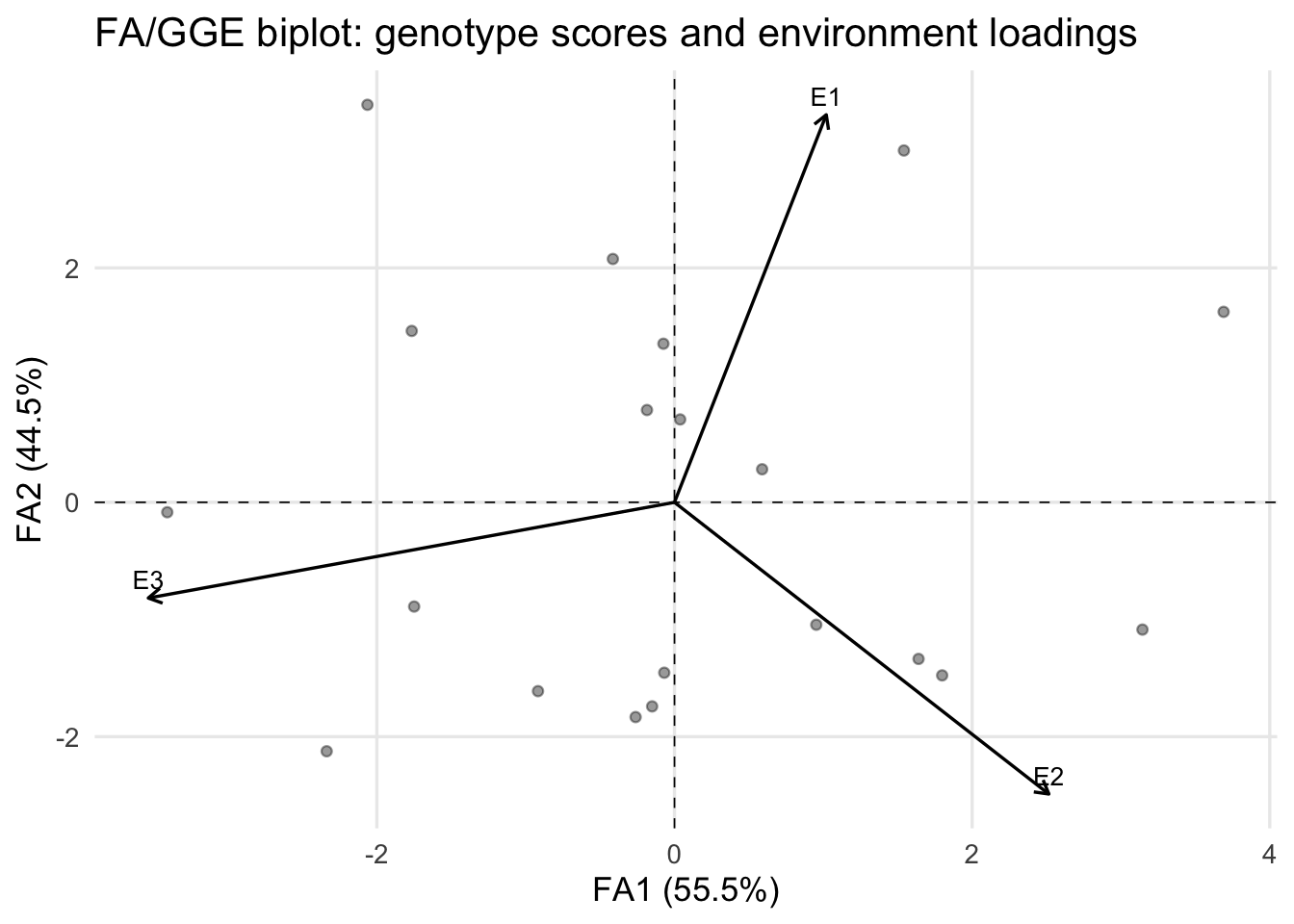
fa_biplot(fa_model, type = "which_won_where")

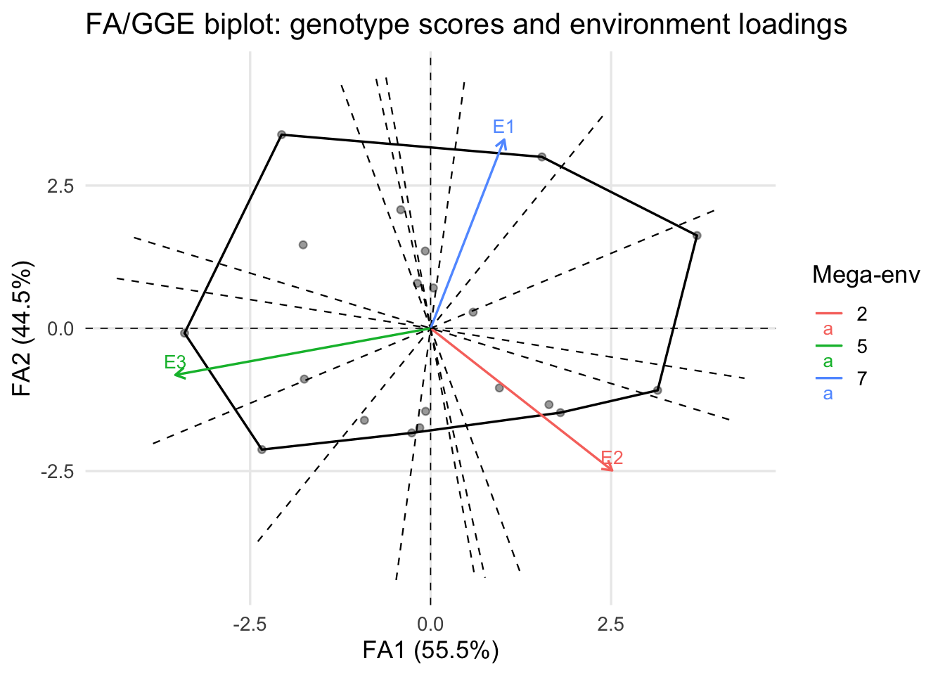
fa_heatmap(fa_model)

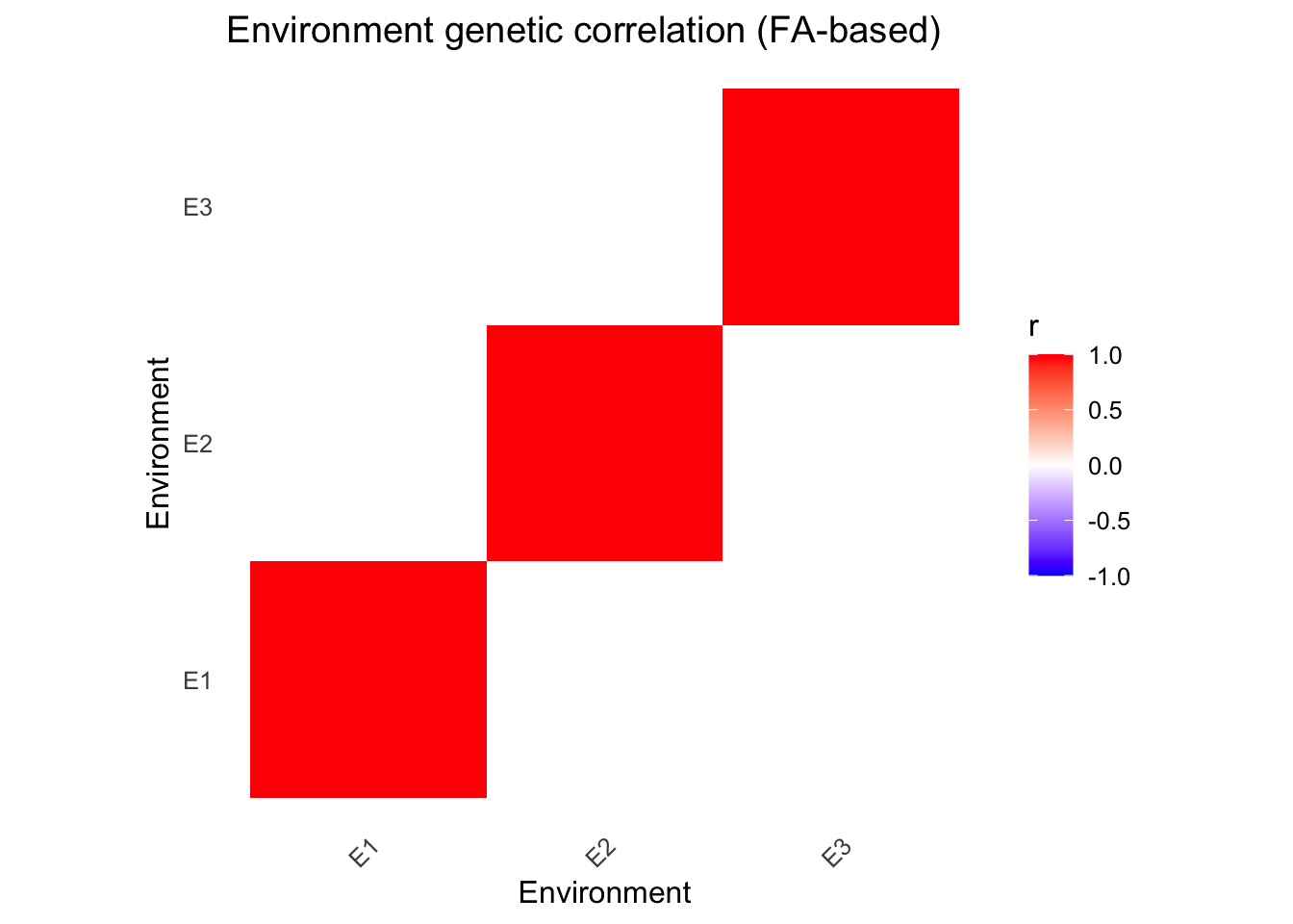
# Extract environment correlations
fa_env_cor(fa_model)
             E1           E2           E3
E1 1.000000e+00 2.253465e-14 2.253464e-14
E2 2.253465e-14 1.000000e+00 4.506688e-14
E3 2.253464e-14 4.506688e-14 1.000000e+00
# Reliability estimates
fa_reliability(fa_model)
   geno env         blup       se      pev  var_env reliability
1   G01  E1   7.76446633 18.21492 197370.6 4437.611           0
2   G02  E1  -0.67666849 18.21514 197375.4 4437.611           0
3   G03  E1   4.18935571 18.22352 197557.0 4437.611           0
4   G04  E1  -8.59831775 18.22352 197557.0 4437.611           0
5   G05  E1  16.10555048 18.22500 197589.2 4437.611           0
6   G06  E1  20.26744882 18.22500 197589.2 4437.611           0
7   G07  E1  -4.37516375 18.20491 197153.7 4437.611           0
8   G08  E1   4.25653605 18.20491 197153.7 4437.611           0
9   G09  E1 -11.14964159 18.20287 197109.6 4437.611           0
10  G10  E1  -4.84037536 18.20287 197109.6 4437.611           0
11  G11  E1 -16.58236399 18.20287 197109.6 4437.611           0
12  G12  E1 -11.03960703 18.20287 197109.6 4437.611           0
13  G13  E1   2.70244363 18.20491 197153.7 4437.611           0
14  G14  E1   5.34808793 18.20491 197153.7 4437.611           0
15  G15  E1  -5.37377101 18.22500 197589.2 4437.611           0
16  G16  E1 -10.41954420 18.22500 197589.2 4437.611           0
17  G17  E1  -8.32977427 18.22352 197557.0 4437.611           0
18  G18  E1  11.35664246 18.22352 197557.0 4437.611           0
19  G19  E1  16.05904086 18.21514 197375.4 4437.611           0
20  G20  E1  -6.62142511 18.21514 197375.4 4437.611           0
21  G01  E2  -6.25531319 18.21494 197371.0 4437.612           0
22  G02  E2  18.70842985 18.21516 197375.8 4437.612           0
23  G03  E2  -2.93347984 18.22353 197557.4 4437.612           0
24  G04  E2   6.07621387 18.22353 197557.4 4437.612           0
25  G05  E2   9.22922326 18.22502 197589.6 4437.612           0
26  G06  E2  -6.33608228 18.22502 197589.6 4437.612           0
27  G07  E2   8.80883117 18.20492 197154.1 4437.612           0
28  G08  E2  -4.27426303 18.20492 197154.1 4437.612           0
29  G09  E2   6.88270781 18.20288 197109.9 4437.612           0
30  G10  E2  13.13581743 18.20288 197109.9 4437.612           0
31  G11  E2  -1.04068785 18.20288 197109.9 4437.612           0
32  G12  E2   3.00428774 18.20288 197109.9 4437.612           0
33  G13  E2   1.37390772 18.20492 197154.1 4437.612           0
34  G14  E2 -14.24390095 18.20492 197154.1 4437.612           0
35  G15  E2  14.45490564 18.22502 197589.6 4437.612           0
36  G16  E2   6.97489333 18.22502 197589.6 4437.612           0
37  G17  E2  -3.85278747 18.22353 197557.4 4437.612           0
38  G18  E2 -10.94551802 18.22353 197557.4 4437.612           0
39  G19  E2 -24.03085888 18.21516 197375.8 4437.612           0
40  G20  E2 -14.73905417 18.21516 197375.8 4437.612           0
41  G01  E3  -1.47438396 18.21494 197371.0 4437.613           0
42  G02  E3 -18.03152530 18.21516 197375.8 4437.613           0
43  G03  E3  -1.25562123 18.22353 197557.4 4437.613           0
44  G04  E3   2.52211745 18.22353 197557.4 4437.613           0
45  G05  E3 -25.33490690 18.22502 197589.6 4437.613           0
46  G06  E3 -13.93141203 18.22502 197589.6 4437.613           0
47  G07  E3  -4.43353401 18.20492 197154.1 4437.613           0
48  G08  E3   0.01778946 18.20492 197154.1 4437.613           0
49  G09  E3   4.26719175 18.20288 197109.9 4437.613           0
50  G10  E3  -8.29534210 18.20288 197109.9 4437.613           0
51  G11  E3  17.62316620 18.20288 197109.9 4437.613           0
52  G12  E3   8.03570324 18.20288 197109.9 4437.613           0
53  G13  E3  -4.07605301 18.20492 197154.1 4437.613           0
54  G14  E3   8.89603214 18.20492 197154.1 4437.613           0
55  G15  E3  -9.08117538 18.22502 197589.6 4437.613           0
56  G16  E3   3.44500408 18.22502 197589.6 4437.613           0
57  G17  E3  12.18295168 18.22353 197557.4 4437.613           0
58  G18  E3  -0.41108424 18.22353 197557.4 4437.613           0
59  G19  E3   7.97205696 18.21516 197375.8 4437.613           0
60  G20  E3  21.36083776 18.21516 197375.8 4437.613           0
fa_reliability_by_env(fa_model)
  env mean_reliability  n
1  E1                0 20
2  E2                0 20
3  E3                0 20
# Factor scores and loadings
fa_geno_scores(fa_model)
   geno         FA1         FA2            method
1   G01 -0.07430727  1.35320989 svd_from_ge_blups
2   G02  3.14463984 -1.08623221 svd_from_ge_blups
3   G03  0.03808185  0.70707267 svd_from_ge_blups
4   G04 -0.06862734 -1.45418159 svd_from_ge_blups
5   G05  3.68993234  1.62516399 svd_from_ge_blups
6   G06  1.54176417  3.00198635 svd_from_ge_blups
7   G07  0.95292860 -1.04470064 svd_from_ge_blups
8   G08 -0.18483763  0.78738085 svd_from_ge_blups
9   G09 -0.26119695 -1.83256024 svd_from_ge_blups
10  G10  1.64008687 -1.33650882 svd_from_ge_blups
11  G11 -2.33703499 -2.12434220 svd_from_ge_blups
12  G12 -0.91706031 -1.61135520 svd_from_ge_blups
13  G13  0.58893280  0.28200084 svd_from_ge_blups
14  G14 -1.76554018  1.46230897 svd_from_ge_blups
15  G15  1.79864126 -1.47693761 svd_from_ge_blups
16  G16 -0.15029916 -1.74150272 svd_from_ge_blups
17  G17 -1.74939550 -0.88961294 svd_from_ge_blups
18  G18 -0.41393083  2.07633652 svd_from_ge_blups
19  G19 -2.06327526  3.39200925 svd_from_ge_blups
20  G20 -3.40822723 -0.08473759 svd_from_ge_blups
fa_env_loadings(fa_model)
     FA1          FA2
E1 1e-05 0.000000e+00
E2 1e-05 9.999469e-06
E3 1e-05 9.999464e-06

Key Differences Summary

Aspect Mandala Sommer
Syntax Simple formula interface More verbose
Heritability Built-in h2_estimates() Manual calculation
Spatial models AR1, P-splines, variograms Via custom covariance
GBLUP GM() + mandala_gp() vsr(Gu=)
FA models FA() with biplots/heatmaps Manual setup
Cross-validation mandala_gp_cv() Manual
Multi-trait (multivariate) No Yes
Speed Fast Moderate

When to Use Each

Use Mandala when:

  • Standard field trial designs
  • Spatial modeling (AR1 or P-splines)
  • Single-trait GBLUP workflows
  • Factor-analytic G×E with visualization
  • Cross-validation for genomic prediction
  • Quick heritability estimates

Use Sommer when:

  • Multi-trait genomic prediction
  • Complex custom covariance structures
  • Marker-based models beyond GBLUP
  • Already established sommer workflows

Additional Resources

Session Information

sessionInfo()
R version 4.5.2 (2025-10-31)
Platform: aarch64-apple-darwin20
Running under: macOS Tahoe 26.2

Matrix products: default
BLAS:   /System/Library/Frameworks/Accelerate.framework/Versions/A/Frameworks/vecLib.framework/Versions/A/libBLAS.dylib 
LAPACK: /Library/Frameworks/R.framework/Versions/4.5-arm64/Resources/lib/libRlapack.dylib;  LAPACK version 3.12.1

locale:
[1] en_US.UTF-8/en_US.UTF-8/en_US.UTF-8/C/en_US.UTF-8/en_US.UTF-8

time zone: America/New_York
tzcode source: internal

attached base packages:
[1] stats     graphics  grDevices utils     datasets  methods   base     

other attached packages:
[1] tidyr_1.3.2    ggplot2_4.0.2  dplyr_1.2.0    sommer_4.4.4   enhancer_1.1.0
[6] crayon_1.5.3   MASS_7.3-65    Matrix_1.7-4   mandala_1.0.1 

loaded via a namespace (and not attached):
 [1] gtable_0.3.6       jsonlite_2.0.0     compiler_4.5.2     tidyselect_1.2.1  
 [5] Rcpp_1.1.1         scales_1.4.0       yaml_2.3.12        fastmap_1.2.0     
 [9] lattice_0.22-7     R6_2.6.1           labeling_0.4.3     generics_0.1.4    
[13] knitr_1.51         htmlwidgets_1.6.4  tibble_3.3.1       pillar_1.11.1     
[17] RColorBrewer_1.1-3 rlang_1.1.7        xfun_0.56          S7_0.2.1          
[21] otel_0.2.0         cli_3.6.5          withr_3.0.2        magrittr_2.0.4    
[25] digest_0.6.39      grid_4.5.2         lifecycle_1.0.5    vctrs_0.7.1       
[29] evaluate_1.0.5     glue_1.8.0         farver_2.1.2       purrr_1.2.1       
[33] rmarkdown_2.30     tools_4.5.2        pkgconfig_2.0.3    htmltools_0.5.9