library(mandala)
library(SpATS)
library(dplyr)
library(ggplot2)Comparison: Mandala vs SpATS
P-spline spatial analysis for field trials
Overview
This tutorial compares the mandala package with the SpATS package for spatial analysis of field trials. Both packages support two-dimensional P-spline spatial correction, so they can be compared on the same field-trial data. Their implementations are similar in intent, but you should not expect numerically identical fits.
NoteWhat you’ll learn
- How Mandala’s
pspline2D(...)formula term compares to SpATS’sPSANOVA() - Side-by-side spatial model fitting
- Variogram diagnostics in both packages
- Fitted value comparison and validation
- When to use each package
Background
SpATS Package
- Purpose: Spatial analysis of field trials using P-splines
- Key Features:
- PSANOVA spatial smoothing
- Built-in spatial diagnostics
- Genotype as fixed or random
- Effective dimension calculations
- Primary Use: Spatial correction in breeding trials
Mandala Package
- Purpose: Comprehensive field trial analysis
- Key Features:
pspline2D(...)formula term for P-spline spatial modeling insidemandala()- AR1×AR1 spatial correlation structures
- Interactive variogram diagnostics
- Integration with GBLUP and FA models
- Primary Use: Field trial analysis with multiple spatial options
Loading Packages
Example 1: Wheat Trial Data
We’ll use the built-in wheatdata from SpATS to compare both approaches on the same trial.
Data Setup
data("wheatdata", package = "SpATS")

# Prepare data for both packages
wheatdata$row.num <- as.numeric(wheatdata$row)
wheatdata$col.num <- as.numeric(wheatdata$col)
wheatdata$yield   <- as.numeric(wheatdata$yield)
wheatdata$row     <- as.factor(wheatdata$row)
wheatdata$col     <- as.factor(wheatdata$col)
wheatdata$rep     <- as.factor(wheatdata$rep)

str(wheatdata)
'data.frame': 330 obs. of 9 variables:
$ yield : num 483 526 557 564 498 510 344 600 466 370 ...
$ geno : Factor w/ 107 levels "1","2","3","4",..: 4 10 17 16 21 32 33 34 72 74 ...
$ rep : Factor w/ 3 levels "1","2","3": 1 1 1 1 1 1 1 1 1 1 ...
$ row : Factor w/ 22 levels "1","2","3","4",..: 1 2 3 4 5 6 7 8 9 10 ...
$ col : Factor w/ 15 levels "1","2","3","4",..: 1 1 1 1 1 1 1 1 1 1 ...
$ rowcode: Factor w/ 2 levels "1","2": 2 2 1 2 2 1 2 2 1 2 ...
$ colcode: Factor w/ 4 levels "1","2","3","4": 1 1 1 1 1 1 1 1 1 1 ...
$ row.num: num 1 2 3 4 5 6 7 8 9 10 ...
$ col.num: num 1 1 1 1 1 1 1 1 1 1 ...head(wheatdata) yield geno rep row col rowcode colcode row.num col.num
1 483 4 1 1 1 2 1 1 1
2 526 10 1 2 1 2 1 2 1
3 557 17 1 3 1 1 1 3 1
4 564 16 1 4 1 2 1 4 1
5 498 21 1 5 1 2 1 5 1
6 510 32 1 6 1 1 1 6 1Visualize Field Layout
ggplot(wheatdata, aes(x = col.num, y = row.num, fill = yield)) +
  geom_tile() +
  scale_fill_gradient2(low = "#2E6B8A", mid = "#FAF8F5", high = "#9B5B5B",
                       midpoint = mean(wheatdata$yield)) +
  coord_equal() +
  theme_minimal() +
  labs(title = "Wheat Trial - Raw Yield",
       x = "Column", y = "Row", fill = "Yield")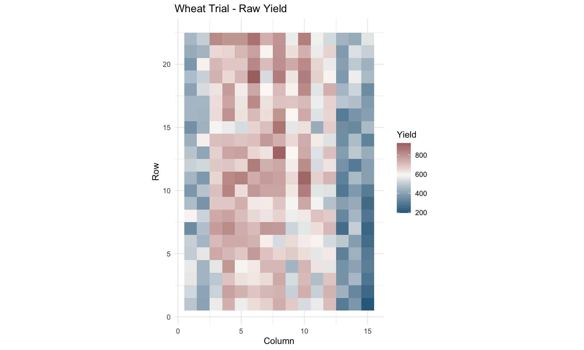
SpATS Analysis
spats_fit <- SpATS(
  response           = "yield",
  genotype           = "geno",
  genotype.as.random = FALSE,
  spatial            = ~ PSANOVA(row.num, col.num,
                                 nseg   = c(10, 20),
                                 degree = c(3, 3),
                                 pord   = c(2, 2)),
  data               = wheatdata
)
Effective dimensions
-------------------------
It. Deviance f(row.num) f(col.num)f(row.num):col.numrow.num:f(col.num)f(row.num):f(col.num)
1 1089936.925340 2.301 5.377 2.212 4.669 13.093
2 2259.016100 2.092 6.669 1.312 3.887 10.805
3 2244.207735 1.929 8.244 0.731 3.234 8.987
4 2217.738426 1.824 10.179 0.275 2.702 7.796
5 2177.035873 1.788 11.936 0.065 2.341 7.516
6 2155.880798 1.768 12.643 0.013 2.181 8.128
7 2154.137260 1.704 12.762 0.003 2.102 8.794
8 2154.011058 1.632 12.777 0.001 2.055 9.299
9 2153.953448 1.566 12.779 0.000 2.026 9.675
10 2153.918651 1.508 12.779 0.000 2.009 9.957
11 2153.897223 1.459 12.780 0.000 2.000 10.168
12 2153.884068 1.418 12.780 0.000 1.997 10.329
13 2153.876082 1.386 12.780 0.000 1.997 10.450
14 2153.871289 1.361 12.780 0.000 2.000 10.543
15 2153.868429 1.342 12.780 0.000 2.003 10.615
16 2153.866719 1.328 12.780 0.000 2.008 10.670
17 2153.865682 1.318 12.781 0.000 2.013 10.714
18 2153.865039 1.310 12.781 0.000 2.017 10.748
Timings:
SpATS 0.084 seconds
All process 0.11 secondssummary(spats_fit)
Spatial analysis of trials with splines

Response:                   yield
Genotypes (as fixed):       geno
Spatial:                    ~PSANOVA(row.num, col.num, nseg = c(10, 20), degree = c(3, 3), pord = c(2, 2))


Number of observations:        330
Number of missing data:        0
Effective dimension:           136.86
Deviance:                      2153.865

Dimensions:
                          Effective     Model     Nominal     Ratio     Type
geno                          106.0       106         106      1.00        F
Intercept                       1.0         1           1      1.00        F
row.num                         1.0         1           1      1.00        S
col.num                         1.0         1           1      1.00        S
col.numrow.num                  1.0         1           1      1.00        S
f(row.num)                      1.3        11          11      0.12        S
f(col.num)                     12.8        21          21      0.61        S
f(row.num):col.num              0.0        11          11      0.00        S
row.num:f(col.num)              2.0        21          21      0.10        S
f(row.num):f(col.num)          10.7       231         231      0.05        S

Total                         136.9       405         405      0.34
Residual                      193.1
Nobs                            330

Type codes: F 'Fixed'    R 'Random'    S 'Smooth/Semiparametric'
SpATS Diagnostics
plot(spats_fit)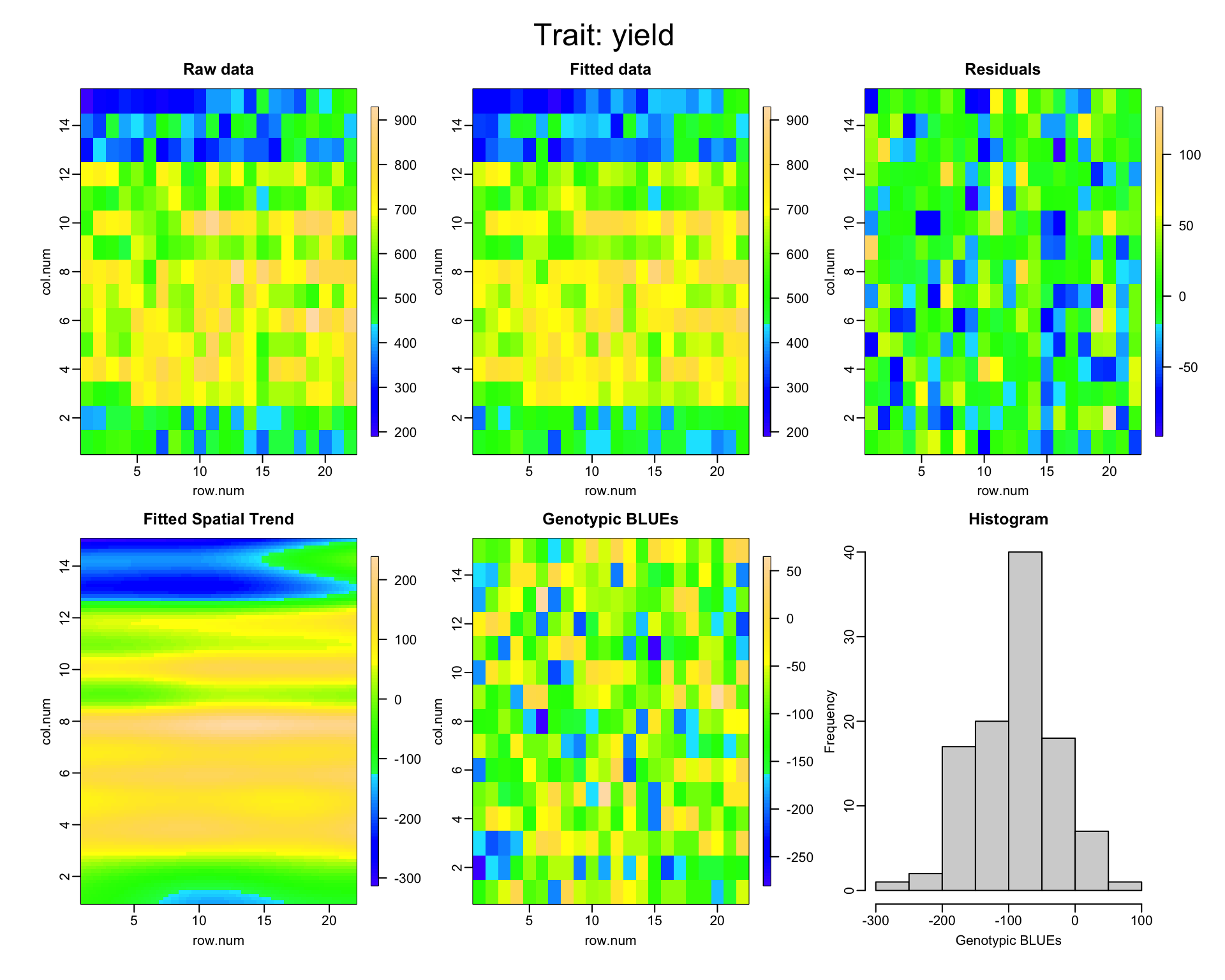
SpATS Variogram
plot(variogram(spats_fit))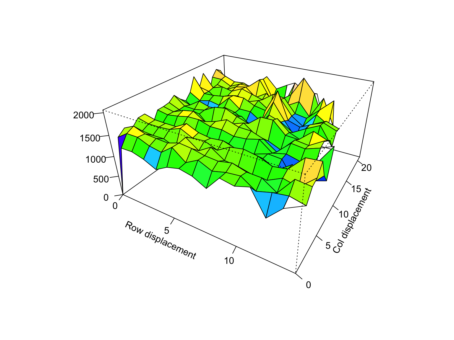
Mandala Analysis
P-spline Model (Comparable Mandala Specification)
# Mandala P-spline specification comparable to SpATS PSANOVA
spline_fit <- mandala(
  fixed  = yield ~ geno,
  random = ~ row.num + col.num + row.num:col.num +
             pspline2D(row.num, col.num,
                       nseg   = c(10, 20),
                       degree = c(3, 3),
                       pord   = c(2, 2)),
  data   = wheatdata,
  verbose = FALSE
)

summary(spline_fit)
Model statement:
mandala(fixed = yield ~ geno, random = ~row.num + col.num + row.num:col.num +
pspline2D(row.num, col.num, nseg = c(10, 20), degree = c(3,
3), pord = c(2, 2)), data = wheatdata, verbose = FALSE)
Variance Components:
component estimate std.error z.ratio bound %ch
row.num 430.2966 204.9152 2.0998764171 P NA
col.num 11422.6580 4675.9774 2.4428385928 P NA
row.num:col.num 1792.6537 144020.1488 0.0124472421 P NA
f(row.num) 4222.0470 5401.3258 0.7816686333 P NA
f(col.num) 6122.4948 9694.8129 0.6315227318 P NA
f(row.num):col.num 4253.1487 5576.7158 0.7626618994 P NA
row.num:f(col.num) 4611.7143 5931.9165 0.7774408619 P NA
f(row.num):f(col.num) 1833.7378 606.3034 3.0244558191 P NA
R.sigma2 103.8410 144020.1488 0.0007210175 P NA
Fixed Effects (BLUEs) [first 5]:
effect estimate std.error z.ratio
(Intercept) 675.54915 40.58509 16.6452538
geno2 -30.02955 41.08700 -0.7308771
geno3 -54.25540 42.04151 -1.2905198
geno4 -128.99994 44.85092 -2.8761940
geno5 -66.19822 42.92704 -1.5421101
Converged: TRUE | Iterations: 10
Random Effects (BLUPs) [first 5]:
random level estimate std.error z.ratio
row.num 1 0.01283462 20.11666 0.0006380094
row.num 2 9.20648130 13.54070 0.6799118162
row.num 3 0.70125340 13.57497 0.0516578108
row.num 4 -12.12422819 13.38103 -0.9060758018
row.num 5 12.63204145 13.41348 0.9417420654
logLik: -1342.980 AIC: 2703.960 BIC: 2734.624 logLik_Trunc: -1138.057The pspline2D(...) term is part of the mandala() formula syntax. It targets the same kind of two-dimensional P-spline spatial correction as SpATS::PSANOVA(), but the two packages do not guarantee identical parameterization or identical fitted values.
Mandala Spatial Diagnostics
# Spatial fitted value plot
plot_mandala_spatial(spline_fit, wheatdata,
                     response = "yield",
                     geno     = "geno",
                     row      = "row",
                     col      = "col")
Notes:
- The predictions are obtained by averaging across the hypertable
  calculated from model terms constructed solely from factors in
  the averaging and classify sets.
- The simple averaging set: (none)
- The ignored set: row.num:col.num, f(row.num), f(col.num), f(row.num):col.num, row.num:f(col.num), f(row.num):f(col.num)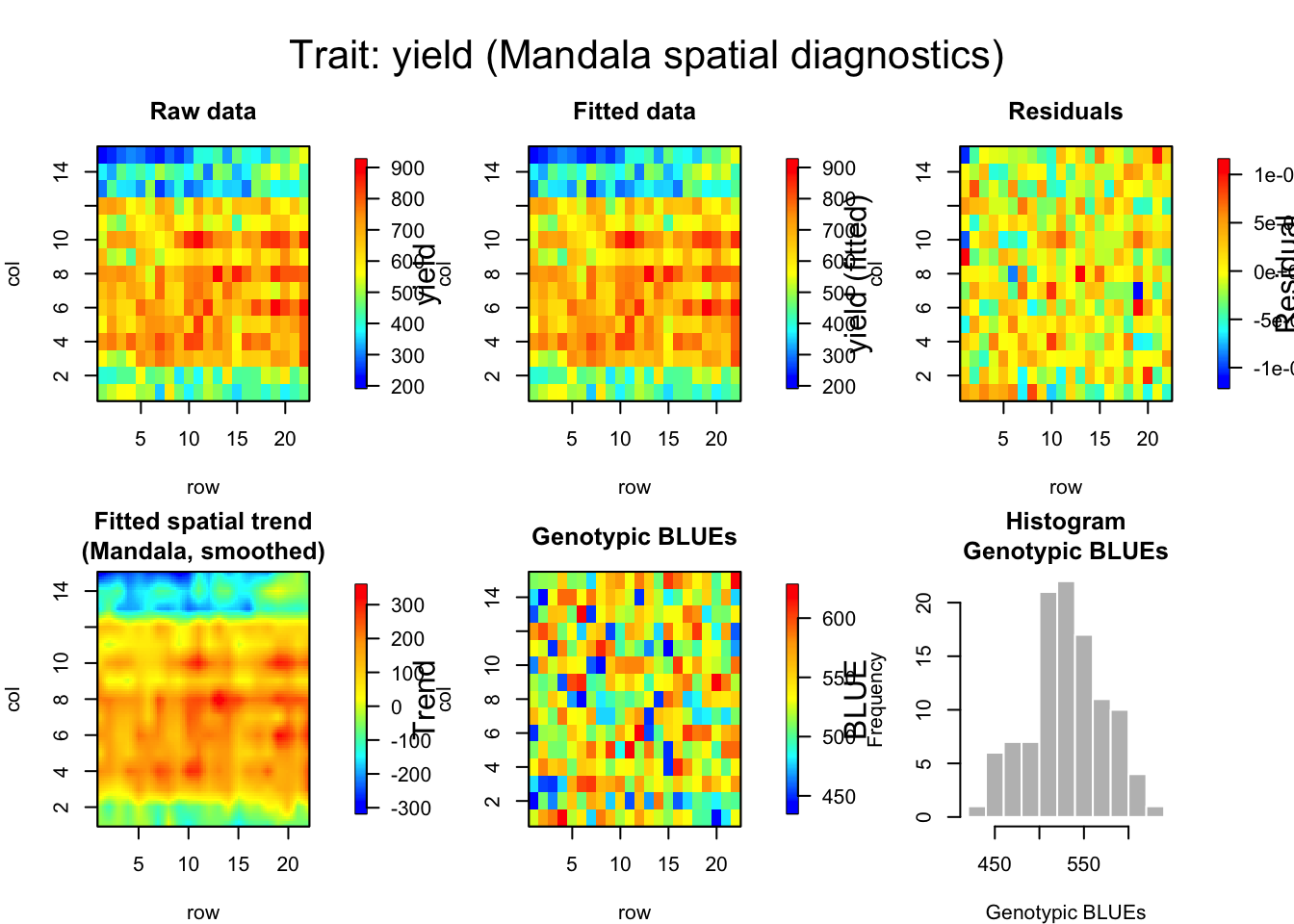
Mandala Variogram Options
# Static 3D mesh
mandala_variogram(spline_fit, data = wheatdata,
                  lag_width = 1, plot_type = "3d")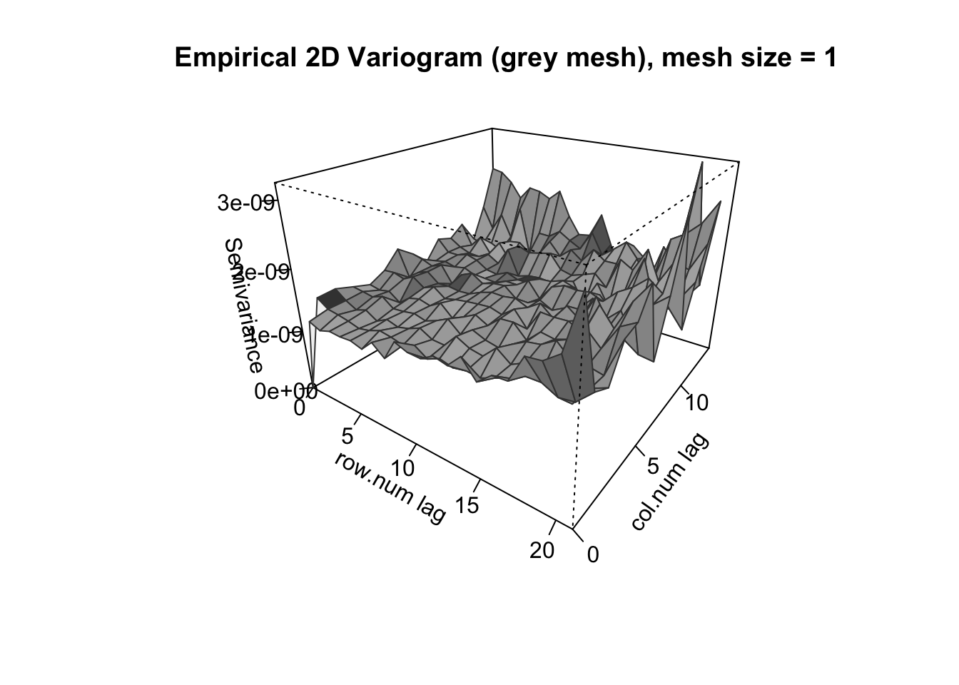
# 2D lag vs semivariance
mandala_variogram(spline_fit, data = wheatdata,
                  lag_width = 2, plot_type = "2d")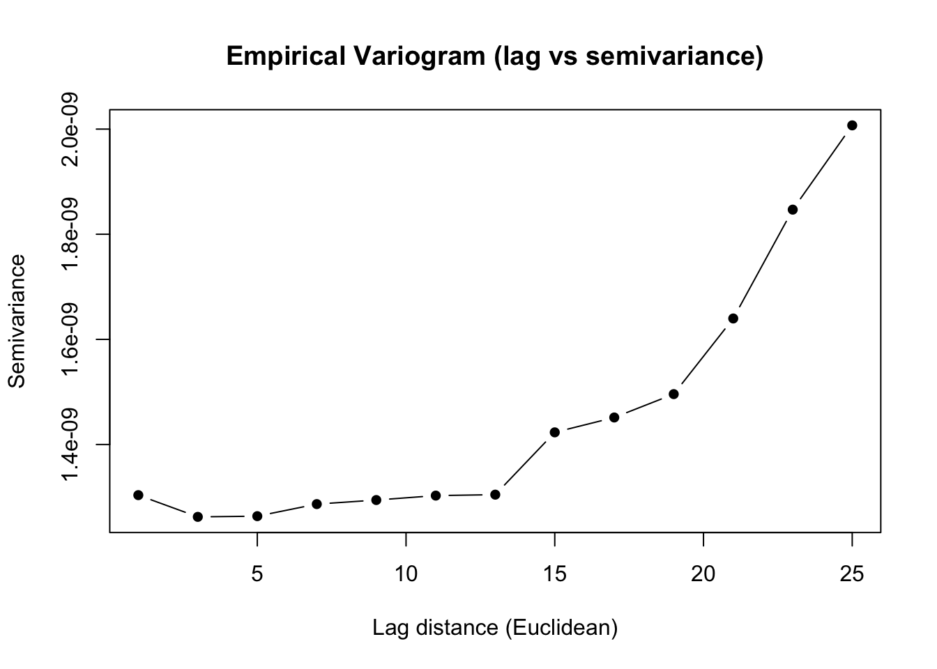
# Interactive Plotly variogram
library(plotly)
mandala_variogram(spline_fit, data = wheatdata,
                  lag_width    = 1,
                  plot_type    = "dynamic",
                  empirical_na = "smooth",
                  overlay      = "ar1xar1")
Alternative: AR1 Spatial Model
Mandala also supports AR1 correlation structures, which SpATS does not:
# AR1×AR1 spatial correlation
ar1_fit <- mandala(
  fixed  = yield ~ geno,
  random = ~ ar1(row) + ar1(col) + ar1(row):ar1(col),
  data   = wheatdata,
  verbose = FALSE
)
Zlst[[3]] dimensions: 330x330summary(ar1_fit)Model statement:
mandala(fixed = yield ~ geno, random = ~ar1(row) + ar1(col) +
ar1(row):ar1(col), data = wheatdata, verbose = FALSE)
Variance Components:
component estimate std.error z.ratio bound %ch
ar1(row) 809.1309566 388.5417862 2.082481 P NA
rho.ar1(row) 0.3656464 0.2634864 1.387724 P NA
ar1(col) 9733.0895992 1617.0734685 6.018953 P NA
rho.ar1(col) 0.9500000 0.0752517 12.624300 B NA
ar1(row):ar1(col) 2089.2092851 540.4125308 3.865953 P NA
rho.row.col.1 0.2113991 0.1805995 1.170541 P NA
rho.row.col.2 0.6646716 0.1307389 5.083961 P NA
R.sigma2 1185.4409293 462.0376181 2.565681 P NA
Fixed Effects (BLUEs) [first 5]:
effect estimate std.error z.ratio
(Intercept) 560.93380 90.44528 6.201913
geno2 -37.26906 39.78923 -0.936662
geno3 -79.61364 42.83845 -1.858462
geno4 -124.64943 42.60802 -2.925492
geno5 -97.46382 42.18750 -2.310253
Converged: TRUE | Iterations: 7
Random Effects (BLUPs) [first 5]:
random level estimate std.error z.ratio
ar1(row) 1 -6.052136 16.25523 -0.3723193
ar1(row) 2 -11.321963 15.93199 -0.7106434
ar1(row) 3 -25.261593 16.32902 -1.5470363
ar1(row) 4 -34.106965 16.43449 -2.0753284
ar1(row) 5 -6.774268 16.55608 -0.4091710
logLik: -1304.521 AIC: 2625.042 BIC: 2652.300 logLik_Trunc: -1099.598# Compare variograms
mandala_variogram(ar1_fit, data = wheatdata,
lag_width = 1,
plot_type = "dynamic",
overlay = "ar1xar1")Comparing Fitted Values
When both models are fit, you can assess how closely they agree:
# Extract fitted values
fitted_spats   <- as.numeric(spats_fit$fitted)
fitted_mandala <- as.numeric(spline_fit$fitted)

# Correlation
cor_fit <- cor(fitted_spats, fitted_mandala)
cat(sprintf("Correlation: %.4f\n", cor_fit))
Correlation: 0.9716# RMSE of difference
rmse_diff <- sqrt(mean((fitted_spats - fitted_mandala)^2))
cat(sprintf("RMSE difference: %.4f\n", rmse_diff))RMSE difference: 36.3305# Scatter plot
comp_df <- data.frame(
SpATS = fitted_spats,
Mandala = fitted_mandala
)
ggplot(comp_df, aes(x = SpATS, y = Mandala)) +
geom_point(alpha = 0.5, color = "#5D4E6D") +
geom_abline(slope = 1, intercept = 0, color = "#9B5B5B", linetype = "dashed") +
theme_minimal() +
labs(title = "SpATS vs Mandala Fitted Values",
x = "SpATS Fitted", y = "Mandala Fitted")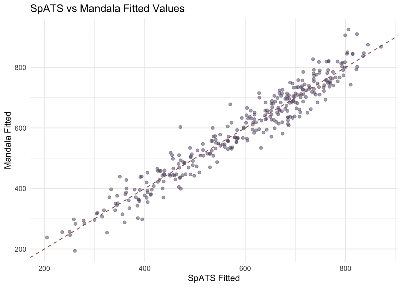
On the wheatdata example under mandala 1.1.0, the fitted values are close but not identical. That is expected: Mandala and SpATS use different implementations and optimization paths even when the spatial specifications are intended to be comparable.
Key Differences Summary
| Aspect | Mandala | SpATS |
|---|---|---|
| P-spline syntax | pspline2D(...) inside random = ~ ... |
PSANOVA() inside spatial = ~ ... |
| AR1 spatial | ar1(row) + ar1(col) |
Not supported |
| Variograms | 2D, 3D, interactive | 2D only |
| Genotype effects | Fixed or random | Fixed or random |
| Genomic models | GM() for GBLUP |
Not supported |
| FA G×E models | FA() |
Not supported |
| MET integration | by(env): syntax |
Single trial focus |
| Diagnostics | plot_mandala_spatial(), mandala_variogram(), mandala_diagnostic_plots() |
plot(), variogram() |
When to Use Each
Use Mandala when:
- Need both P-spline AND AR1 options
- Integrating spatial with GBLUP
- Multi-environment trials with spatial
- Interactive variogram exploration
- Factor-analytic G×E + spatial
Use SpATS when:
- Single-trial P-spline analysis
- Established SpATS workflow
- Effective dimensions important
- Need SpATS-specific outputs
- Want the canonical SpATS PSANOVA implementation
Additional Resources
- SpATS: https://cran.r-project.org/package=SpATS
- Mandala: https://listoagriculture.com/products
- Rodríguez-Álvarez et al. (2018) - SpATS methodology
Session Information
sessionInfo()R version 4.5.2 (2025-10-31)
Platform: aarch64-apple-darwin20
Running under: macOS Tahoe 26.1
Matrix products: default
BLAS: /System/Library/Frameworks/Accelerate.framework/Versions/A/Frameworks/vecLib.framework/Versions/A/libBLAS.dylib
LAPACK: /Library/Frameworks/R.framework/Versions/4.5-arm64/Resources/lib/libRlapack.dylib; LAPACK version 3.12.1
locale:
[1] en_US.UTF-8/en_US.UTF-8/en_US.UTF-8/C/en_US.UTF-8/en_US.UTF-8
time zone: America/New_York
tzcode source: internal
attached base packages:
[1] stats graphics grDevices utils datasets methods base
other attached packages:
[1] plotly_4.11.0 ggplot2_4.0.0 dplyr_1.1.4 SpATS_1.0-19 mandala_1.1.0
loaded via a namespace (and not attached):
[1] Matrix_1.7-4 gtable_0.3.6 jsonlite_2.0.0 compiler_4.5.2
[5] maps_3.4.3 tidyselect_1.2.1 Rcpp_1.1.0 splines2_0.5.4
[9] tidyr_1.3.1 scales_1.4.0 yaml_2.3.10 fastmap_1.2.0
[13] lattice_0.22-7 R6_2.6.1 labeling_0.4.3 generics_0.1.4
[17] knitr_1.50 htmlwidgets_1.6.4 dotCall64_1.2 tibble_3.3.0
[21] pillar_1.11.1 RColorBrewer_1.1-3 rlang_1.1.6 xfun_0.54
[25] S7_0.2.0 lazyeval_0.2.2 viridisLite_0.4.2 cli_3.6.5
[29] withr_3.0.2 magrittr_2.0.4 crosstalk_1.2.2 digest_0.6.37
[33] grid_4.5.2 spam_2.11-3 lifecycle_1.0.4 fields_17.1
[37] vctrs_0.6.5 evaluate_1.0.5 glue_1.8.0 data.table_1.17.8
[41] farver_2.1.2 purrr_1.1.0 httr_1.4.7 rmarkdown_2.30
[45] tools_4.5.2 pkgconfig_2.0.3 htmltools_0.5.8.1