library(mandala)
library(dplyr)
library(ggplot2)Two-Stage MET Analysis
Single-stage vs two-stage workflows for multi-environment trials
Overview
Multi-environment trials (MET) can be analyzed using either single-stage or two-stage approaches. Each has trade-offs:
| Approach | Advantages | Disadvantages |
|---|---|---|
| Single-stage | Fully models all data jointly; optimal if model is correct | Computationally intensive; complex variance structures |
| Two-stage | Computationally efficient; modular workflow | May lose information if Stage 1 uncertainty not propagated |
Mandala supports both approaches and provides tools to properly propagate uncertainty from Stage 1 to Stage 2 using variance-covariance matrices (RMAT).
NoteLearning Objectives
- Fit single-stage MET models with different variance structures
- Implement the two-stage workflow using
stage1_prep(),mandala_stage1(), andstage1_bundle() - Propagate BLUE uncertainty to Stage 2 using
vcov(RMAT) - Calculate heritability at both stages
- Compare single-stage and two-stage results
Data Setup
We’ll use simulated MET data with genotypes evaluated across multiple environments. Each environment has a randomized complete block design with spatial row/column structure.
# Simulate MET data
set.seed(42)

n_env <- 4
n_geno <- 50
n_rep <- 2
n_row <- 10
n_col <- 10

# Create base data structure
df <- expand.grid(
  env = paste0("E", 1:n_env),
  geno = paste0("G", sprintf("%03d", 1:n_geno)),
  rep = 1:n_rep
)

# Assign spatial positions within each env:rep
df <- df %>%
  group_by(env, rep) %>%
  mutate(
    row = rep(1:n_row, length.out = n()),
    col = rep(1:n_col, each = n_row)[1:n()]
  ) %>%
  ungroup()

# Simulate effects
env_effects <- rnorm(n_env, mean = 0, sd = 5)
names(env_effects) <- paste0("E", 1:n_env)

geno_effects <- rnorm(n_geno, mean = 0, sd = 3)
names(geno_effects) <- paste0("G", sprintf("%03d", 1:n_geno))

# GxE interaction
gxe_effects <- matrix(rnorm(n_env * n_geno, mean = 0, sd = 2),
                      nrow = n_geno, ncol = n_env)
rownames(gxe_effects) <- names(geno_effects)
colnames(gxe_effects) <- names(env_effects)

# Build response
df <- df %>%
  mutate(
    yld = 100 +
      env_effects[as.character(env)] +
      geno_effects[as.character(geno)] +
      sapply(1:n(), function(i) gxe_effects[as.character(geno[i]), as.character(env[i])]) +
      rnorm(n(), mean = 0, sd = 2)  # residual
  )

# Convert to factors
df$env <- as.factor(df$env)
df$geno <- as.factor(df$geno)
df$rep <- as.factor(df$rep)
df$row <- as.factor(df$row)
df$col <- as.factor(df$col)
df$block <- df$rep  # alias for consistency

head(df)
# A tibble: 6 × 7
env geno rep row col yld block
<fct> <fct> <fct> <fct> <fct> <dbl> <fct>
1 E1 G001 1 1 1 111. 1
2 E2 G001 1 1 1 95.0 1
3 E3 G001 1 1 1 101. 1
4 E4 G001 1 1 1 102. 1
5 E1 G002 1 2 1 105. 1
6 E2 G002 1 2 1 96.3 1 # Check data structure
df %>%
group_by(env) %>%
summarise(
n_obs = n(),
n_geno = n_distinct(geno),
mean_yld = mean(yld),
sd_yld = sd(yld)
)# A tibble: 4 × 5
env n_obs n_geno mean_yld sd_yld
<fct> <int> <int> <dbl> <dbl>
1 E1 100 50 107. 3.86
2 E2 100 50 96.5 4.45
3 E3 100 50 102. 4.59
4 E4 100 50 103. 3.80Single-Stage MET Analysis
Single-stage analysis fits all data in one model. We demonstrate four model variants with different fixed/random specifications.
Model 1: Genotype and GxE Fixed
Estimate fixed genotype means and fixed GxE interaction. Design effects are random.
MET_model1 <- mandala(
  fixed  = yld ~ env + geno + env:geno,
  random = ~ env:rep + env:row + env:col,
  data   = df
)
Initial data rows: 400
Final data rows after NA handling: 400 --- Starting EM Warmup ---
EM Warmup: starting theta:
env:rep 12.71 env:row 12.71 env:col 12.71 R.sigma2 15.89
EM iter 1: logLik=-560.2753; theta: env:rep 9.543 env:row 12.71 env:col 12.71 R.sigma2 1.844
EM iter 2: logLik=-524.9387; theta: env:rep 7.201 env:row 12.71 env:col 12.71 R.sigma2 1.845
EM iter 3: logLik=-524.3725; theta: env:rep 5.41 env:row 12.71 env:col 12.71 R.sigma2 1.844
EM iter 4: logLik=-523.8144; theta: env:rep 4.067 env:row 12.71 env:col 12.71 R.sigma2 1.844
EM iter 5: logLik=-523.2521; theta: env:rep 3.059 env:row 12.71 env:col 12.71 R.sigma2 1.844
EM Warmup: ending theta:
env:rep 3.059 env:row 12.71 env:col 12.71 R.sigma2 1.844
--- EM Warmup Complete. Starting AI-REML ---Starting AI-REML logLik = -522.6940
Iter LogLik Sigma2 DF wall Restrained
1 -504.6371 2.287 200 14:56:04 ( 0 restrained)
2 -494.0647 2.836 200 14:56:05 ( 0 restrained)
3 -489.8827 3.452 200 14:56:05 ( 0 restrained)
4 -489.2608 3.838 200 14:56:05 ( 0 restrained)
5 -489.0886 3.965 200 14:56:05 ( 0 restrained)
6 -488.7539 3.930 200 14:56:05 ( 0 restrained)
7 -488.3893 3.842 200 14:56:05 ( 0 restrained)
8 -488.0805 3.768 200 14:56:05 ( 0 restrained)
9 -487.8057 3.731 200 14:56:05 ( 0 restrained)
10 -487.5397 3.726 200 14:56:06 ( 0 restrained)
11 -487.2805 3.735 200 14:56:06 ( 0 restrained)
12 -487.0315 3.748 200 14:56:06 ( 0 restrained)
13 -486.7934 3.756 200 14:56:06 ( 0 restrained)
14 -486.5662 3.759 200 14:56:06 ( 0 restrained)
15 -486.3505 3.758 200 14:56:06 ( 0 restrained)
16 -486.1472 3.756 200 14:56:06 ( 0 restrained)
17 -485.9570 3.755 200 14:56:06 ( 0 restrained)
18 -485.7805 3.754 200 14:56:07 ( 0 restrained)
19 -485.6180 3.754 200 14:56:07 ( 0 restrained)
20 -485.4694 3.754 200 14:56:07 ( 0 restrained)
21 -485.3346 3.754 200 14:56:07 ( 0 restrained)
22 -485.2132 3.755 200 14:56:07 ( 0 restrained)
23 -485.1047 3.755 200 14:56:07 ( 0 restrained)
24 -485.0083 3.755 200 14:56:07 ( 0 restrained)
25 -484.9232 3.755 200 14:56:08 ( 0 restrained)
26 -484.8486 3.755 200 14:56:08 ( 0 restrained)
27 -484.7835 3.755 200 14:56:08 ( 0 restrained)
Froze env:rep at 1.000009e-05
28 -484.7270 3.755 200 14:56:08 ( 1 restrained)
29 -484.3893 3.755 200 14:56:08 ( 1 restrained)
30 -484.3893 3.755 200 14:56:08 ( 1 restrained)
Converged at iter 30 by tolerance(s): delta_theta=0.00e+00, delta_loglik=0.00e+00
Main AI-REML Loop finished. Combining results.summary(MET_model1)Model statement:
mandala(fixed = yld ~ env + geno + env:geno, random = ~env:rep +
env:row + env:col, data = df)
Variance Components:
component estimate std.error z.ratio bound %ch
env:rep 1.000009e-05 5.364309e-02 1.864190e-04 B NA
env:row 4.331926e+00 1.565893e+14 2.766426e-14 P NA
env:col 1.072798e+01 8.520183e+13 1.259125e-13 P NA
R.sigma2 3.754529e+00 3.792645e-01 9.899502e+00 P NA
Fixed Effects (BLUEs) [first 5]:
effect estimate std.error z.ratio
(Intercept) 109.6442609 4.112474 26.6613873
envE2 -13.9398242 5.816446 -2.3966223
envE3 -6.6710219 5.816446 -1.1469241
envE4 -7.2589418 5.816446 -1.2480030
genoG002 -0.6096677 3.523308 -0.1730384
Converged: TRUE | Iterations: 30
Random Effects (BLUPs) [first 5]:
random level estimate std.error z.ratio
env:rep E1.1 2.871378e-05 0.003162187 0.0090803549
env:rep E2.1 3.399284e-07 0.003162187 0.0001074979
env:rep E3.1 -1.287100e-05 0.003162187 -0.0040702857
env:rep E4.1 -1.811673e-05 0.003162187 -0.0057291786
env:rep E1.2 -2.871305e-05 0.003162187 -0.0090801233
logLik: -484.389 AIC: 976.779 BIC: 989.972 logLik_Trunc: -300.602Model 2: Genotype Fixed, GxE Random
Estimate fixed genotype effects while treating GxE as random. Common for inference on genotype main effects.
MET_model2 <- mandala(
  fixed  = yld ~ env + geno,
  random = ~ env:geno + env:rep + env:row + env:col,
  data   = df
)
Initial data rows: 400
Final data rows after NA handling: 400
--- Starting EM Warmup ---
EM Warmup: starting theta:
env:geno 12.71 env:rep 12.71 env:row 12.71 env:col 12.71 R.sigma2 15.89
EM iter 1: logLik=-1005.6104; theta: env:geno 9.987 env:rep 9.543 env:row 9.226 env:col 9.308 R.sigma2 2.9
EM iter 2: logLik=-916.3746; theta: env:geno 8.354 env:rep 7.201 env:row 6.901 env:col 6.929 R.sigma2 3.436
EM iter 3: logLik=-904.9885; theta: env:geno 6.864 env:rep 5.412 env:row 5.126 env:col 5.143 R.sigma2 3.011
EM iter 4: logLik=-898.4885; theta: env:geno 5.771 env:rep 4.072 env:row 3.862 env:col 3.852 R.sigma2 3.072
EM iter 5: logLik=-891.6048; theta: env:geno 4.951 env:rep 3.066 env:row 2.949 env:col 2.912 R.sigma2 3.081
EM Warmup: ending theta:
env:geno 4.951 env:rep 3.066 env:row 2.949 env:col 2.912 R.sigma2 3.081
--- EM Warmup Complete. Starting AI-REML ---Starting AI-REML logLik = -886.4365
Iter LogLik Sigma2 DF wall Restrained
1 -880.5759 3.620 347 14:56:09 ( 0 restrained)
2 -877.8699 4.159 347 14:56:09 ( 0 restrained)
3 -876.2515 4.215 347 14:56:09 ( 0 restrained)
4 -874.1225 4.046 347 14:56:09 ( 0 restrained)
5 -872.2457 3.852 347 14:56:09 ( 0 restrained)
6 -870.7499 3.730 347 14:56:09 ( 0 restrained)
7 -869.4727 3.689 347 14:56:10 ( 0 restrained)
8 -868.3304 3.699 347 14:56:10 ( 0 restrained)
9 -867.3102 3.727 347 14:56:10 ( 0 restrained)
10 -866.3988 3.750 347 14:56:10 ( 0 restrained)
11 -865.5792 3.762 347 14:56:10 ( 0 restrained)
12 -864.8407 3.764 347 14:56:10 ( 0 restrained)
13 -864.1780 3.761 347 14:56:10 ( 0 restrained)
14 -863.5868 3.757 347 14:56:10 ( 0 restrained)
15 -863.0615 3.754 347 14:56:11 ( 0 restrained)
16 -862.5961 3.753 347 14:56:11 ( 0 restrained)
17 -862.1841 3.753 347 14:56:11 ( 0 restrained)
18 -861.8198 3.754 347 14:56:11 ( 0 restrained)
19 -861.4982 3.754 347 14:56:11 ( 0 restrained)
20 -861.2147 3.755 347 14:56:11 ( 0 restrained)
21 -860.9655 3.755 347 14:56:11 ( 0 restrained)
22 -860.7472 3.755 347 14:56:12 ( 0 restrained)
23 -860.5566 3.755 347 14:56:12 ( 0 restrained)
24 -860.3907 3.755 347 14:56:12 ( 0 restrained)
25 -860.2469 3.755 347 14:56:12 ( 0 restrained)
26 -860.1225 3.755 347 14:56:12 ( 0 restrained)
27 -860.0152 3.755 347 14:56:12 ( 0 restrained)
Froze env:rep at 9.999599e-06
Froze env:row at 1.000033e-05
Froze env:col at 1.000158e-05
28 -859.9229 3.755 347 14:56:12 ( 3 restrained)
29 -859.3845 3.755 347 14:56:13 ( 3 restrained)
30 -859.3845 3.755 347 14:56:13 ( 3 restrained)
Converged at iter 30 by tolerance(s): delta_theta=0.00e+00, delta_loglik=0.00e+00
Main AI-REML Loop finished. Combining results.summary(MET_model2)Model statement:
mandala(fixed = yld ~ env + geno, random = ~env:geno + env:rep +
env:row + env:col, data = df)
Variance Components:
component estimate std.error z.ratio bound %ch
env:geno 4.383172e+00 0.8727878 5.022036e+00 P NA
env:rep 9.999599e-06 0.0536432 1.864094e-04 B NA
env:row 1.000033e-05 0.3810006 2.624755e-05 B NA
env:col 1.000158e-05 0.2694103 3.712396e-05 B NA
R.sigma2 3.754539e+00 0.3792652 9.899509e+00 P NA
Fixed Effects (BLUEs) [first 5]:
effect estimate std.error z.ratio
(Intercept) 107.8318845 1.2879953 83.7207122
envE2 -10.6439443 0.5004328 -21.2694776
envE3 -5.5060711 0.5004328 -11.0026182
envE4 -4.4688854 0.5004328 -8.9300410
genoG002 -0.3650888 1.7692144 -0.2063565
Converged: TRUE | Iterations: 30
Random Effects (BLUPs) [first 5]:
random level estimate std.error z.ratio
env:geno E1.G001 1.2725634 1.458609 0.8724497
env:geno E2.G001 -1.0396545 1.458610 -0.7127709
env:geno E3.G001 0.4528869 1.458610 0.3104922
env:geno E4.G001 -0.6853295 1.458610 -0.4698513
env:geno E1.G002 1.0999023 1.458625 0.7540680
logLik: -859.384 AIC: 1728.769 BIC: 1748.016 logLik_Trunc: -540.513Model 3: Environment Fixed, Genotype and GxE Random
Partition genetic variance across environments. Useful for heritability and variance component estimation.
MET_model3 <- mandala(
  fixed  = yld ~ env,
  random = ~ geno + env:geno + env:rep + env:row + env:col,
  data   = df
)
Initial data rows: 400
Final data rows after NA handling: 400
--- Starting EM Warmup ---
EM Warmup: starting theta:
geno 12.71 env:geno 12.71 env:rep 12.71 env:row 12.71 env:col 12.71 R.sigma2 15.89
EM iter 1: logLik=-1142.4222; theta: geno 10 env:geno 9.818 env:rep 9.543 env:row 8.584 env:col 8.581 R.sigma2 5.779
EM iter 2: logLik=-1056.9317; theta: geno 8.182 env:geno 8.109 env:rep 7.201 env:row 6.082 env:col 5.987 R.sigma2 6.696
EM iter 3: logLik=-1053.1028; theta: geno 6.931 env:geno 6.649 env:rep 5.42 env:row 4.347 env:col 4.23 R.sigma2 6.191
EM iter 4: logLik=-1040.4371; theta: geno 6.077 env:geno 5.586 env:rep 4.086 env:row 3.2 env:col 3.066 R.sigma2 6.364
EM iter 5: logLik=-1035.2517; theta: geno 5.503 env:geno 4.785 env:rep 3.084 env:row 2.417 env:col 2.278 R.sigma2 6.418
EM Warmup: ending theta:
geno 5.503 env:geno 4.785 env:rep 3.084 env:row 2.417 env:col 2.278 R.sigma2 6.418
--- EM Warmup Complete. Starting AI-REML ---Starting AI-REML logLik = -1030.8455
Iter LogLik Sigma2 DF wall Restrained
1 -1015.3260 4.878 396 14:56:13 ( 0 restrained)
2 -1007.4047 3.707 396 14:56:14 ( 0 restrained)
3 -1006.4582 3.235 396 14:56:14 ( 0 restrained)
4 -1004.7878 3.255 396 14:56:14 ( 0 restrained)
5 -1002.7457 3.473 396 14:56:14 ( 0 restrained)
6 -1001.3215 3.683 396 14:56:15 ( 0 restrained)
7 -1000.2559 3.801 396 14:56:15 ( 0 restrained)
8 -999.2703 3.831 396 14:56:15 ( 0 restrained)
9 -998.3311 3.812 396 14:56:15 ( 0 restrained)
10 -997.4763 3.779 396 14:56:15 ( 0 restrained)
11 -996.7199 3.755 396 14:56:16 ( 0 restrained)
12 -996.0536 3.745 396 14:56:16 ( 0 restrained)
13 -995.4646 3.745 396 14:56:16 ( 0 restrained)
14 -994.9419 3.749 396 14:56:16 ( 0 restrained)
15 -994.4761 3.753 396 14:56:17 ( 0 restrained)
16 -994.0599 3.755 396 14:56:17 ( 0 restrained)
17 -993.6881 3.756 396 14:56:17 ( 0 restrained)
18 -993.3569 3.756 396 14:56:17 ( 0 restrained)
19 -993.0628 3.755 396 14:56:18 ( 0 restrained)
20 -992.8028 3.755 396 14:56:18 ( 0 restrained)
21 -992.5737 3.754 396 14:56:18 ( 0 restrained)
22 -992.3726 3.754 396 14:56:18 ( 0 restrained)
23 -992.1965 3.754 396 14:56:18 ( 0 restrained)
24 -992.0429 3.754 396 14:56:19 ( 0 restrained)
25 -991.9093 3.755 396 14:56:19 ( 0 restrained)
Froze env:col at 9.998505e-06
26 -991.7935 3.755 396 14:56:19 ( 1 restrained)
Froze env:row at 1.000017e-05
27 -991.6288 3.755 396 14:56:19 ( 2 restrained)
Froze env:rep at 9.999991e-06
28 -991.4426 3.755 396 14:56:20 ( 3 restrained)
29 -991.1023 3.755 396 14:56:20 ( 3 restrained)
30 -991.1023 3.755 396 14:56:20 ( 3 restrained)
Converged at iter 30 by tolerance(s): delta_theta=0.00e+00, delta_loglik=0.00e+00
Main AI-REML Loop finished. Combining results.summary(MET_model3)Model statement:
mandala(fixed = yld ~ env, random = ~geno + env:geno + env:rep +
env:row + env:col, data = df)
Variance Components:
component estimate std.error z.ratio bound %ch
geno 1.028426e+01 2.40204348 4.281463e+00 P NA
env:geno 4.405181e+00 0.87506846 5.034099e+00 P NA
env:rep 9.999991e-06 0.05364342 1.864160e-04 B NA
env:row 1.000017e-05 0.38122685 2.623155e-05 B NA
env:col 9.998505e-06 0.26957022 3.709054e-05 B NA
R.sigma2 3.754539e+00 0.37926674 9.899469e+00 P NA
Fixed Effects (BLUEs) [first 5]:
effect estimate std.error z.ratio
(Intercept) 107.191690 0.5756216 186.219030
envE2 -10.643944 0.5013116 -21.232191
envE3 -5.506071 0.5013116 -10.983330
envE4 -4.468885 0.5013116 -8.914386
Converged: TRUE | Iterations: 30
Random Effects (BLUPs) [first 5]:
random level estimate std.error z.ratio
geno G001 0.5555188 1.241354 0.4475104
geno G002 0.2386548 1.241354 0.1922537
geno G003 3.4283639 1.241354 2.7617941
geno G004 -1.4838819 1.241354 -1.1953738
geno G005 3.2728545 1.241354 2.6365201
logLik: -991.102 AIC: 1994.205 BIC: 2018.093 logLik_Trunc: -627.203Model 4: All Random (Variance Partitioning)
Full variance component model for partitioning total variance.
MET_model4 <- mandala(
  fixed  = yld ~ 1,
  random = ~ env + geno + env:geno + env:rep + env:row + env:col,
  data   = df
)
Initial data rows: 400
Final data rows after NA handling: 400
--- Starting EM Warmup ---
EM Warmup: starting theta:
env 12.71 geno 12.71 env:geno 12.71 env:rep 12.71 env:row 12.71 env:col 12.71 R.sigma2 15.89
EM iter 1: logLik=-1151.8243; theta: env 11.18 geno 10 env:geno 9.817 env:rep 9.158 env:row 8.568 env:col 8.52 R.sigma2 9.362
EM iter 2: logLik=-1093.5325; theta: env 9.951 geno 8.182 env:geno 8.108 env:rep 6.707 env:row 6.065 env:col 5.92 R.sigma2 10.31
EM iter 3: logLik=-1089.8760; theta: env 9.038 geno 6.924 env:geno 6.709 env:rep 4.954 env:row 4.367 env:col 4.194 R.sigma2 10.05
EM iter 4: logLik=-1079.3846; theta: env 8.415 geno 6.055 env:geno 5.673 env:rep 3.698 env:row 3.243 env:col 3.056 R.sigma2 10.27
EM iter 5: logLik=-1074.5132; theta: env 8.042 geno 5.459 env:geno 4.878 env:rep 2.785 env:row 2.474 env:col 2.288 R.sigma2 10.39
EM Warmup: ending theta:
env 8.042 geno 5.459 env:geno 4.878 env:rep 2.785 env:row 2.474 env:col 2.288 R.sigma2 10.39
--- EM Warmup Complete. Starting AI-REML ---Starting AI-REML logLik = -1070.4971
Iter LogLik Sigma2 DF wall Restrained
1 -1046.3475 7.899 399 14:56:21 ( 0 restrained)
2 -1028.0175 6.003 399 14:56:21 ( 0 restrained)
3 -1016.0388 4.263 399 14:56:21 ( 0 restrained)
4 -1013.8728 3.318 399 14:56:22 ( 0 restrained)
5 -1013.4529 3.105 399 14:56:22 ( 0 restrained)
6 -1011.2657 3.288 399 14:56:22 ( 0 restrained)
7 -1009.5063 3.561 399 14:56:22 ( 0 restrained)
8 -1008.4677 3.757 399 14:56:23 ( 0 restrained)
9 -1007.6300 3.838 399 14:56:23 ( 0 restrained)
10 -1006.8046 3.837 399 14:56:23 ( 0 restrained)
11 -1006.0250 3.802 399 14:56:23 ( 0 restrained)
12 -1005.3324 3.767 399 14:56:24 ( 0 restrained)
13 -1004.7289 3.747 399 14:56:24 ( 0 restrained)
14 -1004.2017 3.742 399 14:56:24 ( 0 restrained)
15 -1003.7384 3.745 399 14:56:25 ( 0 restrained)
16 -1003.3288 3.750 399 14:56:25 ( 0 restrained)
17 -1002.9652 3.754 399 14:56:25 ( 0 restrained)
18 -1002.6419 3.756 399 14:56:25 ( 0 restrained)
19 -1002.3551 3.756 399 14:56:26 ( 0 restrained)
20 -1002.1018 3.756 399 14:56:26 ( 0 restrained)
21 -1001.8792 3.755 399 14:56:26 ( 0 restrained)
22 -1001.6845 3.754 399 14:56:26 ( 0 restrained)
23 -1001.5149 3.754 399 14:56:27 ( 0 restrained)
24 -1001.3675 3.754 399 14:56:27 ( 0 restrained)
25 -1001.2399 3.754 399 14:56:27 ( 0 restrained)
Froze env:col at 1.000161e-05
26 -1001.1296 3.755 399 14:56:28 ( 1 restrained)
Froze env:row at 9.999025e-06
27 -1000.9696 3.755 399 14:56:28 ( 2 restrained)
Froze env:rep at 9.999198e-06
28 -1000.7853 3.755 399 14:56:28 ( 3 restrained)
29 -1000.4768 3.755 399 14:56:28 ( 3 restrained)
30 -1000.4767 3.755 399 14:56:29 ( 3 restrained)
31 -1000.4767 3.755 399 14:56:29 ( 3 restrained)
32 -1000.4767 3.755 399 14:56:29 ( 3 restrained)
Converged at iter 32 by tolerance(s): delta_theta=0.00e+00, delta_loglik=0.00e+00
Main AI-REML Loop finished. Combining results.summary(MET_model4)Model statement:
mandala(fixed = yld ~ 1, random = ~env + geno + env:geno + env:rep +
env:row + env:col, data = df)
Variance Components:
component estimate std.error z.ratio bound %ch
env 1.909128e+01 15.69071594 1.216725e+00 P NA
geno 1.028310e+01 2.40181194 4.281393e+00 P NA
env:geno 4.405217e+00 0.87507272 5.034115e+00 P NA
env:rep 9.999198e-06 0.05364335 1.864014e-04 B NA
env:row 9.999025e-06 0.38122865 2.622842e-05 B NA
env:col 1.000161e-05 0.26957150 3.710189e-05 B NA
R.sigma2 3.754536e+00 0.37926628 9.899472e+00 P NA
Fixed Effects (BLUEs) [first 5]:
effect estimate std.error z.ratio
(Intercept) 102.0366 2.23826 45.58747
Converged: TRUE | Iterations: 32
Random Effects (BLUPs) [first 5]:
random level estimate std.error z.ratio
env E1 5.1213981 2.205983 2.3215948
env E2 -5.4529588 2.205983 -2.4718954
env E3 -0.3486815 2.205983 -0.1580618
env E4 0.6817221 2.205983 0.3090333
geno G001 0.5555093 1.241339 0.4475081
logLik: -1000.477 AIC: 2014.953 BIC: 2042.876 logLik_Trunc: -633.820Two-Stage Workflow
The two-stage approach separates within-environment analysis (Stage 1) from across-environment analysis (Stage 2).
Stage 1: Per-Environment Analysis
Stage 1 fits separate models for each environment, extracting genotype BLUEs and their variance-covariance matrix.
Step 1: Prepare Stage 1 Configuration
s1_prep <- stage1_prep(
 df              = df,
 env_col         = "env",
 s1_fixed        = yld ~ geno,
 s1_random       = ~ rep + row + col,
 s1_classify_term = "geno",
 response_var    = "yld"
)
Step 2: Audit Stage 1 Setup
stage1_audit(df, s1_prep) env rows nonmiss_response nonmiss_id n_id_levels
1 E1 100 100 100 50
2 E2 100 100 100 50
3 E3 100 100 100 50
4 E4 100 100 100 50Step 3: Run Stage 1 Models
MET_stage1_run <- mandala_stage1(
 df   = df,
 prep = s1_prep
)
Notes:
- The predictions are obtained by averaging across the hypertable
  calculated from model terms constructed solely from factors in
  the averaging and classify sets.
- The simple averaging set: (none)
- The ignored set: rep, row, col
Notes:
- The predictions are obtained by averaging across the hypertable
  calculated from model terms constructed solely from factors in
  the averaging and classify sets.
- The simple averaging set: (none)
- The ignored set: rep, row, col
Notes:
- The predictions are obtained by averaging across the hypertable
  calculated from model terms constructed solely from factors in
  the averaging and classify sets.
- The simple averaging set: (none)
- The ignored set: rep, row, col
Notes:
- The predictions are obtained by averaging across the hypertable
  calculated from model terms constructed solely from factors in
  the averaging and classify sets.
- The simple averaging set: (none)
- The ignored set: rep, row, col
Step 4: Report Check
stage1_report_check(MET_stage1_run, df) env fit_present BLUEs_present n_BLUE_rows error_message
1 E1 TRUE TRUE 50 <NA>
2 E2 TRUE TRUE 50 <NA>
3 E3 TRUE TRUE 50 <NA>
4 E4 TRUE TRUE 50 <NA>Step 5: Bundle Stage 1 Outputs
The bundle contains BLUEs and their variance-covariance matrices for Stage 2.
bundle <- stage1_bundle(MET_stage1_run)

# Preview BLUEs
head(bundle$blues)
env id BLUE SE
1 E1 G001 109.6489 2.695147
2 E1 G002 109.0377 2.695300
3 E1 G003 113.4326 2.695300
4 E1 G004 108.8727 2.695300
5 E1 G005 107.4885 2.695300
6 E1 G006 106.9830 2.695300Stage 2: Across-Environment Analysis
Stage 2 analyzes the BLUEs from Stage 1, using vcov(RMAT) to account for BLUE uncertainty.
Step 1: Prepare Stage 2 Data
s2_inputs <- stage2_prep(
 bundle    = bundle,
 df_name   = "stage2_data",
 vcov_name = "RMAT",
 out_env   = "env",
 out_id    = "geno",
 out_resp  = "yld"
)

s2_data <- s2_inputs$stage2_data
RMAT    <- s2_inputs$RMAT

head(s2_data)
env geno yld
1 E1 G001 109.6489
2 E1 G002 109.0377
3 E1 G003 113.4326
4 E1 G004 108.8727
5 E1 G005 107.4885
6 E1 G006 106.9830# Preview RMAT structure (top-left corner)
RMAT[1:5, 1:5]5 x 5 sparse Matrix of class "dsCMatrix"
E1|G001 E1|G002 E1|G003 E1|G004 E1|G005
E1|G001 7.263815 1.636300 1.636300 1.636300 1.636300
E1|G002 1.636300 7.264640 1.636406 1.636406 1.636406
E1|G003 1.636300 1.636406 7.264640 1.636406 1.636406
E1|G004 1.636300 1.636406 1.636406 7.264640 1.636406
E1|G005 1.636300 1.636406 1.636406 1.636406 7.264640Step 2: Align Row IDs
Ensure s2_data rownames match RMAT for proper variance structure alignment.
rownames(s2_data) <- paste0(s2_data$env, "|", s2_data$geno)
s2_data <- s2_data[rownames(RMAT), , drop = FALSE]

# Verify alignment
stopifnot(identical(rownames(s2_data), rownames(RMAT)))
Step 3: Ensure Matrix Format
if (!inherits(RMAT, "Matrix")) {
 RMAT <- Matrix::forceSymmetric(Matrix::Matrix(RMAT, sparse = TRUE))
}
Step 4: Fit Stage 2 Model
MET_stage2_run <- mandala(
 fixed       = yld ~ env,
 random      = ~ geno,
 R_formula   = ~ vcov(RMAT),
 data        = s2_data,
 matrix_list = list(RMAT = RMAT)
)
Initial data rows: 200
Final data rows after NA handling: 200 --- EM Warmup Skipped. Starting AI-REML ---Starting AI-REML logLik = -554.8966
Iter LogLik Sigma2 DF wall Restrained
1 -544.7874 11.399 196 14:56:31 ( 0 restrained)
2 -537.2573 8.664 196 14:56:31 ( 0 restrained)
3 -529.2477 5.217 196 14:56:31 ( 0 restrained)
4 -528.9685 3.034 196 14:56:31 ( 0 restrained)
5 -528.9685 3.034 196 14:56:31 ( 0 restrained)
Converged at iter 5 by tolerance(s): delta_theta=0.00e+00, delta_loglik=0.00e+00
Main AI-REML Loop finished. Combining results.summary(MET_stage2_run)Model statement:
mandala(fixed = yld ~ env, random = ~geno, data = s2_data, matrix_list = list(RMAT = RMAT),
R_formula = ~vcov(RMAT))
Variance Components:
component estimate std.error z.ratio bound %ch
geno 10.202405 2.6120170 3.905949 P NA
R.sigma2 3.033944 0.9498473 3.194139 P NA
Fixed Effects (BLUEs) [first 5]:
effect estimate std.error z.ratio
(Intercept) 107.191648 0.5145133 208.33601
envE2 -10.643971 0.3483644 -30.55413
envE3 -5.506118 0.3483644 -15.80563
envE4 -4.468908 0.3483644 -12.82826
Converged: TRUE | Iterations: 5
Random Effects (BLUPs) [first 5]:
random level estimate std.error z.ratio
geno G001 0.5955164 0.9465325 0.6291558
geno G002 0.2560207 0.9465325 0.2704828
geno G003 3.6784336 0.9465325 3.8862200
geno G004 -1.5921461 0.9465325 -1.6820828
geno G005 3.5115972 0.9465325 3.7099593
logLik: -528.969 AIC: 1061.937 BIC: 1068.493 logLik_Trunc: -348.857Step 5: Extract Predictions
predicted_means <- mandala_predict(MET_stage2_run, classify_term = "geno")
Notes:
- The predictions are obtained by averaging across the hypertable
  calculated from model terms constructed solely from factors in
  the averaging and classify sets.
- The simple averaging set: env, [num mean] head(predicted_means) geno predicted_value std_error
1 G001 102.6324 0.8408617
2 G002 102.2929 0.8408617
3 G003 105.7153 0.8408617
4 G004 100.4448 0.8408617
5 G005 105.5485 0.8408617
6 G006 102.5585 0.8408617Step 6: Calculate Reliability
reliability <- stage2_reliability(
 MET_stage2_run,
 classify_term = "geno",
 preds         = predicted_means
)

head(reliability)
geno predicted_value std_error PEV reliability accuracy weight_invPEV
1 G001 102.6324 0.8408617 0.7070484 0.9306979 0.9647268 1.41433
2 G002 102.2929 0.8408617 0.7070484 0.9306979 0.9647268 1.41433
3 G003 105.7153 0.8408617 0.7070484 0.9306979 0.9647268 1.41433
4 G004 100.4448 0.8408617 0.7070484 0.9306979 0.9647268 1.41433
5 G005 105.5485 0.8408617 0.7070484 0.9306979 0.9647268 1.41433
6 G006 102.5585 0.8408617 0.7070484 0.9306979 0.9647268 1.41433Heritability Estimation
Stage 1 Heritability (Within-Environment)
Calculate heritability for each environment using the Stage 1 bundle.
s1_heritability <- mandala.h2(
 df           = df,
 out          = NULL,
 bundle       = bundle,
 env_col      = "env",
 genotype_col = "geno",
 response_col = "yld",
 h2_fixed     = yld ~ 1,
 h2_random    = ~ geno + rep + row + col,
 em_iters     = 5,
 maxit        = 100,
 tol          = 1e-2,
 verbose      = FALSE
)

s1_heritability
env n_genotypes sigma_g2 sigma_e2 mean_PEV mean_PEVD H2_plot H2_entrymean
1 E1 50 9.239014 5.265611 7.264623 13.43905 0.6369702 0.6068507
2 E2 50 18.660968 3.070977 8.024043 14.60777 0.8586884 0.7850046
3 E3 50 21.298680 3.662298 13.177499 24.19742 0.8532791 0.6906499
4 E4 50 13.256756 3.019129 6.880465 12.54227 0.8145029 0.7404921
H2_Cullis_PEV H2_Cullis_PEVD
1 0.6068507 0.2727009
2 0.7850046 0.6086009
3 0.6906499 0.4319503
4 0.7404921 0.5269481Stage 2 Heritability (Across-Environment)
Calculate broad-sense heritability from the Stage 2 model.
h2_stage2 <- h2_estimates(
 random_mod = MET_stage2_run,
 genotype   = "geno"
)

h2_stage2
variable value
source_random TRUE
source_fixed FALSE
sigma_g2 10.2024051335264
sigma_e2 3.03394444840794
n_rep 4
mean_PEV_BLUP 0.895923811668298
avsed_BLUE NA
vdBLUE_avg NA
H2_Cullis 0.912185038729331
H2_Piepho NA
H2_Plot 0.770786920545766
H2_Standard 0.930800689916115
Note:
Plot and entry mean heritabilities are just the approximation- assuming a single experiment with only 'genotype' and 'error' variance components in the model. For MET, modify the equations and estimate accordinglyVariance Summary
stage2_variance_summary(MET_stage2_run, s2_data, RMAT) Component Variance PVE
1 env NA NA
2 genotype 10.202405 0.4660504
3 g x env 3.033944 0.1385919
4 Stage1.error 8.654854 0.3953576Single vs Two-Stage Comparison
Compare genotype rankings between single-stage (Model 3) and two-stage approaches.
Extract BLUPs
# Single-stage BLUPs
b1 <- subset(MET_model3$BLUPs, random == "geno")[, c("level", "estimate")]
names(b1) <- c("geno", "blup_single")

# Two-stage BLUPs
b2 <- subset(MET_stage2_run$BLUPs, random == "geno")[, c("level", "estimate")]
names(b2) <- c("geno", "blup_two")

# Merge
blup_comparison <- merge(b1, b2, by = "geno")
head(blup_comparison)
geno blup_single blup_two
1 G001 0.5555188 0.5955164
2 G002 0.2386548 0.2560207
3 G003 3.4283639 3.6784336
4 G004 -1.4838819 -1.5921461
5 G005 3.2728545 3.5115972
6 G006 0.4862198 0.5216380Correlation Analysis
cor_blup <- cor(blup_comparison$blup_single, blup_comparison$blup_two,
               use = "complete.obs")
cat("Correlation between single-stage and two-stage BLUPs:", round(cor_blup, 3), "\n")
Correlation between single-stage and two-stage BLUPs: 1 Scatter Plot: BLUPs
ggplot(blup_comparison, aes(x = blup_single, y = blup_two)) +
 geom_point(alpha = 0.6, size = 2) +
 geom_abline(intercept = 0, slope = 1, linetype = "dashed", color = "red") +
 labs(
   title = "Genotype BLUPs: Single-Stage vs Two-Stage",
   subtitle = paste("r =", round(cor_blup, 3)),
   x = "BLUPs (Single-stage MET)",
   y = "BLUPs (Two-stage MET)"
 ) +
 theme_minimal()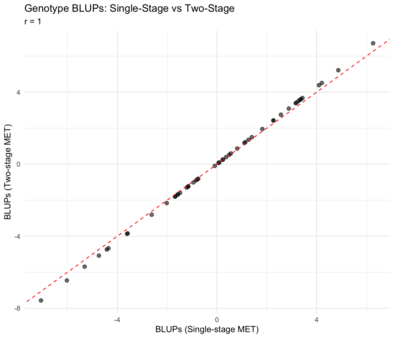
Compare Predicted Means
# Single-stage predictions
p1 <- mandala_predict(MET_model3, classify_term = "geno")
Notes:
- The predictions are obtained by averaging across the hypertable
  calculated from model terms constructed solely from factors in
  the averaging and classify sets.
- The simple averaging set: env, [num mean]
- The ignored set: env:rep, env:row, env:col
p1 <- p1[, c("geno", "predicted_value")]
names(p1) <- c("geno", "pred_single")
# Two-stage predictions
p2 <- predicted_means[, c("geno", "predicted_value")]
names(p2) <- c("geno", "pred_two")
# Merge
pred_comparison <- merge(p1, p2, by = "geno")
cor_pred <- cor(pred_comparison$pred_single, pred_comparison$pred_two,
use = "complete.obs")ggplot(pred_comparison, aes(x = pred_single, y = pred_two)) +
geom_point(alpha = 0.6, size = 2) +
geom_abline(intercept = 0, slope = 1, linetype = "dashed", color = "red") +
labs(
title = "Predicted Means: Single-Stage vs Two-Stage",
subtitle = paste("r =", round(cor_pred, 3)),
x = "Predicted Means (Single-stage)",
y = "Predicted Means (Two-stage)"
) +
theme_minimal()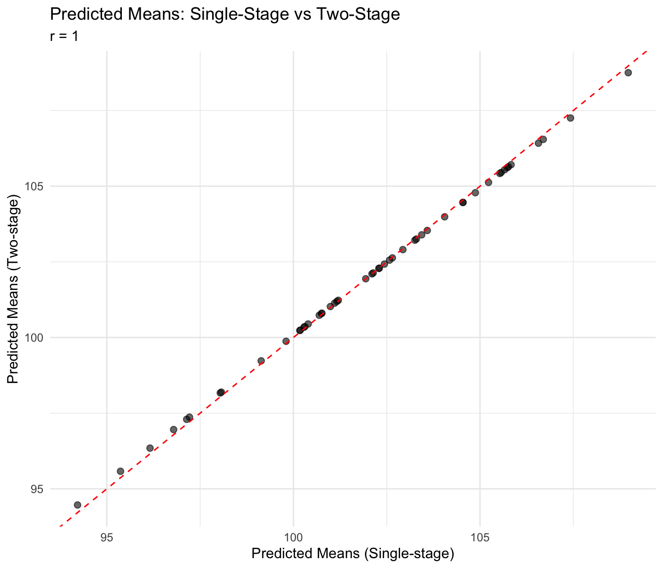
Summary
TipKey Takeaways
- Single-stage models fit all data jointly but can be computationally intensive
- Two-stage workflows are modular and efficient, especially for large METs
- Use
vcov(RMAT)to properly propagate Stage 1 uncertainty to Stage 2 - Both approaches should give similar genotype rankings when properly implemented
- Mandala provides heritability functions for both stages
Next Steps
- Tutorial 07: Two-Stage Genomics — Integrate GBLUP with the two-stage workflow
Session Information
sessionInfo()R version 4.5.2 (2025-10-31)
Platform: aarch64-apple-darwin20
Running under: macOS Tahoe 26.1
Matrix products: default
BLAS: /System/Library/Frameworks/Accelerate.framework/Versions/A/Frameworks/vecLib.framework/Versions/A/libBLAS.dylib
LAPACK: /Library/Frameworks/R.framework/Versions/4.5-arm64/Resources/lib/libRlapack.dylib; LAPACK version 3.12.1
locale:
[1] C.UTF-8/C.UTF-8/C.UTF-8/C/C.UTF-8/C.UTF-8
time zone: America/New_York
tzcode source: internal
attached base packages:
[1] stats graphics grDevices utils datasets methods base
other attached packages:
[1] ggplot2_4.0.0 dplyr_1.1.4 mandala_1.1.0
loaded via a namespace (and not attached):
[1] vctrs_0.6.5 cli_3.6.5 knitr_1.50 rlang_1.1.6
[5] xfun_0.54 generics_0.1.4 S7_0.2.0 splines2_0.5.4
[9] jsonlite_2.0.0 labeling_0.4.3 glue_1.8.0 htmltools_0.5.8.1
[13] scales_1.4.0 rmarkdown_2.30 grid_4.5.2 evaluate_1.0.5
[17] tibble_3.3.0 fastmap_1.2.0 yaml_2.3.10 lifecycle_1.0.4
[21] compiler_4.5.2 codetools_0.2-20 RColorBrewer_1.1-3 htmlwidgets_1.6.4
[25] Rcpp_1.1.0 pkgconfig_2.0.3 farver_2.1.2 lattice_0.22-7
[29] digest_0.6.37 R6_2.6.1 utf8_1.2.6 tidyselect_1.2.1
[33] pillar_1.11.1 magrittr_2.0.4 Matrix_1.7-4 withr_3.0.2
[37] gtable_0.3.6 tools_4.5.2