Comparison: Mandala vs lme4

Field trial analysis vs general-purpose mixed models

Overview

This tutorial compares the mandala package with lme4, the most widely-used R package for mixed models. Where both packages support the same linear mixed model directly, the examples below fit the same structure in both packages. Where Mandala extends beyond base lme4 with field-trial-specific spatial terms and postprocessing, those features are shown as workflow extensions rather than as one-to-one model matches.

What you’ll learn

How the same RCBD and nested mixed models look in Mandala and lme4
Which outputs are directly comparable across the two packages
Where Mandala adds field-trial-specific helpers on top of a standard mixed-model workflow
When differences reflect model targets or workflow scope rather than a disagreement in results

Background

Package	Primary Focus	Best For
lme4	General-purpose	Any discipline
Mandala	Agricultural trials	Field experiments

Loading Packages

library(mandala)
library(lme4)
library(dplyr)
library(ggplot2)

get_mandala_vc <- function(varcomp, term) {
  hits <- which(varcomp$component == term)
  if (length(hits) != 1L) {
    stop("Expected exactly one Mandala variance component for term: ", term)
  }
  varcomp$estimate[hits]
}

get_lme4_vc <- function(varcomp, grp) {
  hits <- which(varcomp$grp == grp)
  if (length(hits) != 1L) {
    stop("Expected exactly one lme4 variance component for group: ", grp)
  }
  varcomp$vcov[hits]
}

Example 1: Basic RCBD

Data Setup

set.seed(321)
n_genotypes <- 12
n_blocks <- 5

rcbd_data <- expand.grid(
  genotype = factor(paste0("G", sprintf("%02d", 1:n_genotypes))),
  block = factor(paste0("B", 1:n_blocks))
)

rcbd_data$yield <- 4500 +
  rnorm(n_genotypes, 0, 20)[as.numeric(rcbd_data$genotype)] +
  rnorm(n_blocks, 0, 10)[as.numeric(rcbd_data$block)] +
  rnorm(nrow(rcbd_data), 0, 15)

head(rcbd_data)

  genotype block    yield
1      G01    B1 4542.286
2      G02    B1 4496.306
3      G03    B1 4503.019
4      G04    B1 4513.249
5      G05    B1 4497.798
6      G06    B1 4522.072

Syntax Comparison

Mandala:

mandala(
  fixed  = yield ~ genotype,
  random = ~ block,
  data   = rcbd_data
)

lme4:

lmer(
  yield ~ genotype + (1|block),
  data = rcbd_data
)

Mandala RCBD

mandala_rcbd <- mandala(
  fixed  = yield ~ genotype,
  random = ~ block,
  data   = rcbd_data,
  verbose = FALSE
)

mandala_rcbd_vc <- mandala_rcbd$varcomp
mandala_rcbd_coef <- mandala_rcbd$BLUEs %>%
  transmute(effect, mandala_estimate = estimate)

print(mandala_rcbd_vc)

  component estimate std.error  z.ratio bound %ch
1     block 129.1804 102.67498 1.258149     P  NA
2  R.sigma2 215.5579  40.79218 5.284295     P  NA

head(mandala_rcbd_coef)

                 effect mandala_estimate
(Intercept) (Intercept)       4529.89386
genotypeG02 genotypeG02        -47.16105
genotypeG03 genotypeG03        -33.39576
genotypeG04 genotypeG04        -19.82680
genotypeG05 genotypeG05        -28.04273
genotypeG06 genotypeG06        -16.66351

lme4 RCBD

lme4_model <- lmer(
  yield ~ genotype + (1|block),
  data = rcbd_data,
  REML = TRUE
)

lme4_rcbd_vc <- as.data.frame(VarCorr(lme4_model))
lme4_rcbd_coef <- tibble(
  effect = names(fixef(lme4_model)),
  lme4_estimate = unname(fixef(lme4_model))
)

print(lme4_rcbd_vc)

       grp        var1 var2     vcov    sdcor
1    block (Intercept) <NA> 125.5453 11.20470
2 Residual        <NA> <NA> 221.6143 14.88671

head(lme4_rcbd_coef)

# A tibble: 6 × 2
  effect      lme4_estimate
  <chr>               <dbl>
1 (Intercept)        4530. 
2 genotypeG02         -47.2
3 genotypeG03         -33.4
4 genotypeG04         -19.8
5 genotypeG05         -28.0
6 genotypeG06         -16.7

RCBD Comparison

rcbd_coef_compare <- inner_join(
  mandala_rcbd_coef,
  lme4_rcbd_coef,
  by = "effect"
)

head(rcbd_coef_compare)

       effect mandala_estimate lme4_estimate
1 (Intercept)       4529.89386    4529.90137
2 genotypeG02        -47.16105     -47.16590
3 genotypeG03        -33.39576     -33.40059
4 genotypeG04        -19.82680     -19.83162
5 genotypeG05        -28.04273     -28.04756
6 genotypeG06        -16.66351     -16.66832

tibble(
  package = c("Mandala", "lme4"),
  block_variance = c(get_mandala_vc(mandala_rcbd_vc, "block"),
                     get_lme4_vc(lme4_rcbd_vc, "block")),
  residual_variance = c(get_mandala_vc(mandala_rcbd_vc, "R.sigma2"),
                        get_lme4_vc(lme4_rcbd_vc, "Residual"))
)

# A tibble: 2 × 3
  package block_variance residual_variance
  <chr>            <dbl>             <dbl>
1 Mandala           129.              216.
2 lme4              126.              222.

What Differs Here

Both packages are fitting the same fixed-genotype RCBD model in this section, so the coefficient and variance-component estimates should be close. The main difference is workflow: Mandala exposes a field-trial-oriented fixed-effect solution table directly through model$BLUEs, while lme4 gives the same fixed-effect information through fixef() and the variance components through VarCorr().

Example 2: Nested Design

Data Setup

set.seed(654)
n_genotypes <- 30
n_complete <- 3

nested_data <- expand.grid(
  genotype = factor(paste0("G", sprintf("%02d", 1:n_genotypes))),
  complete_block = factor(1:n_complete)
)

nested_data$incomplete_block <- factor(
  paste0(nested_data$complete_block, ".",
         rep(1:5, length.out = nrow(nested_data)))
)

nested_data$yield <- 5500 +
  rnorm(n_genotypes, 0, 30)[as.numeric(nested_data$genotype)] +
  rnorm(n_complete, 0, 15)[as.numeric(nested_data$complete_block)] +
  rnorm(nrow(nested_data), 0, 20)

Mandala Nested Design

mandala_nested <- mandala(
  fixed  = yield ~ genotype,
  random = ~ complete_block + complete_block:incomplete_block,
  data   = nested_data,
  verbose = FALSE
)

mandala_nested_vc <- mandala_nested$varcomp
print(mandala_nested_vc)

                        component     estimate std.error      z.ratio bound %ch
1                  complete_block 1.000090e-05  16.69320 5.991001e-07     B  NA
2 complete_block:incomplete_block 2.448528e+01  38.65217 6.334773e-01     P  NA
3                        R.sigma2 3.010141e+02  60.20275 5.000007e+00     P  NA

lme4 Nested Design

lme4_nested <- lmer(
  yield ~ genotype + (1|complete_block) + (1|complete_block:incomplete_block),
  data = nested_data,
  REML = TRUE
)

lme4_nested_vc <- as.data.frame(VarCorr(lme4_nested))
print(lme4_nested_vc)

                              grp        var1 var2        vcov      sdcor
1 complete_block:incomplete_block (Intercept) <NA>  24.4848159  4.9482134
2                  complete_block (Intercept) <NA>   0.7170808  0.8468062
3                        Residual        <NA> <NA> 301.0144193 17.3497671

Nested Design Comparison

tibble(
  package = c("Mandala", "lme4"),
  complete_block_variance = c(get_mandala_vc(mandala_nested_vc, "complete_block"),
                              get_lme4_vc(lme4_nested_vc, "complete_block")),
  incomplete_block_variance = c(get_mandala_vc(mandala_nested_vc, "complete_block:incomplete_block"),
                                get_lme4_vc(lme4_nested_vc, "complete_block:incomplete_block")),
  residual_variance = c(get_mandala_vc(mandala_nested_vc, "R.sigma2"),
                        get_lme4_vc(lme4_nested_vc, "Residual"))
)

# A tibble: 2 × 4
  package complete_block_variance incomplete_block_variance residual_variance
  <chr>                     <dbl>                     <dbl>             <dbl>
1 Mandala               0.0000100                      24.5              301.
2 lme4                  0.717                          24.5              301.

What Differs Here

This example stays within the overlap between the two packages, so the nested-block variance decomposition is directly comparable. When a variance component is near zero, the two optimizers may report slightly different boundary behavior, but the practical conclusion is the same if both fits place little support on that component.

Diagnostics

Both packages support diagnostics, but they package them differently: lme4 exposes fitted values and residuals for general R plotting workflows, while Mandala bundles common field-trial diagnostics into dedicated helpers.

lme4 Diagnostics

diag_data <- data.frame(
  Fitted = fitted(lme4_model),
  Residuals = residuals(lme4_model)
)

p1 <- ggplot(diag_data, aes(x = Fitted, y = Residuals)) +
  geom_point(alpha = 0.6, color = "#5D4E6D") +
  geom_hline(yintercept = 0, linetype = "dashed", color = "#9B5B5B") +
  geom_smooth(se = FALSE, color = "#8B9A6D") +
  theme_minimal() +
  labs(title = "Residuals vs Fitted")

p2 <- ggplot(diag_data, aes(sample = Residuals)) +
  stat_qq(color = "#5D4E6D") +
  stat_qq_line(color = "#9B5B5B") +
  theme_minimal() +
  labs(title = "Normal Q-Q Plot")

gridExtra::grid.arrange(p1, p2, ncol = 2)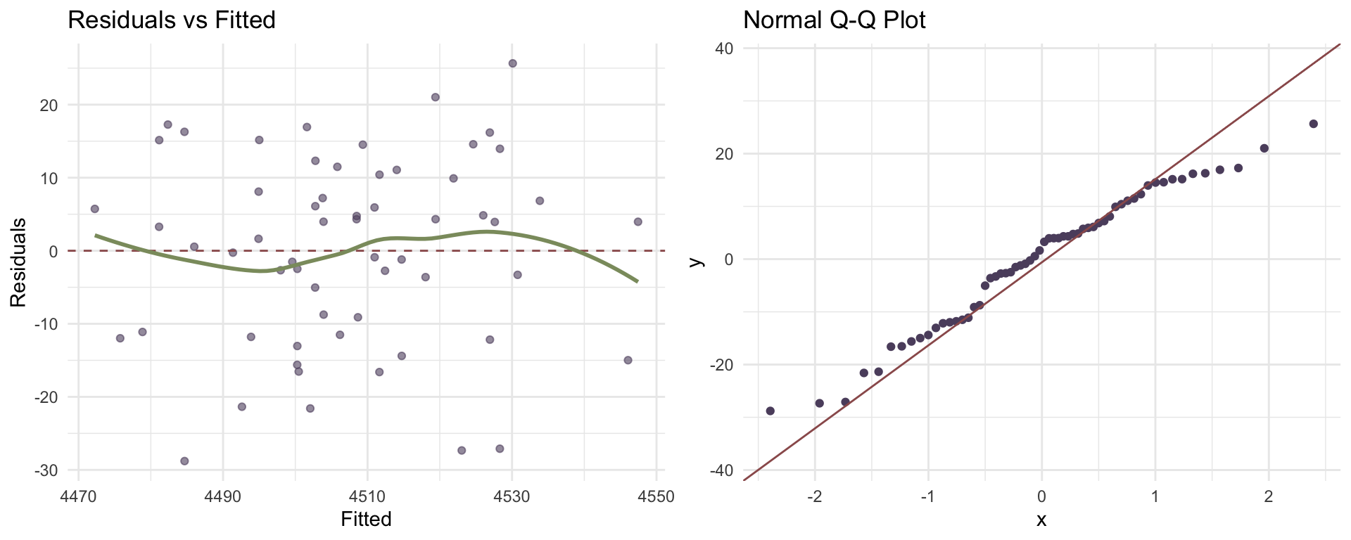

Mandala Diagnostics

# Built-in diagnostic plots for the Mandala RCBD fit
mandala_diagnostic_plots(mandala_rcbd, response = "yield")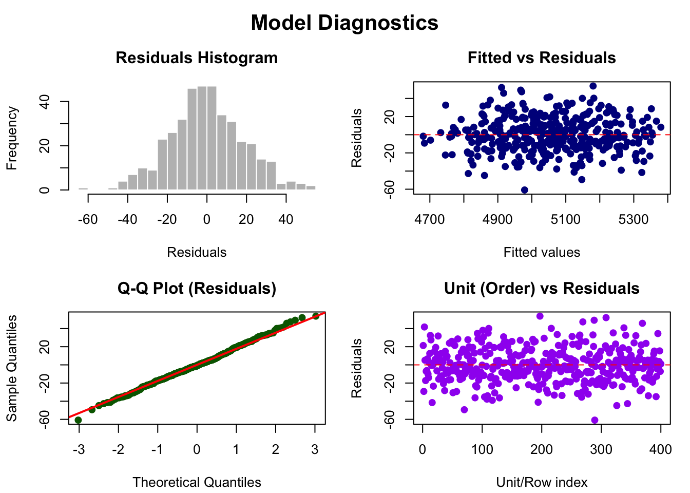

# Includes:
# - Residuals vs fitted
# - Q-Q plot
# - Histogram of residuals
# - Observed vs predicted

Key Differences

Task	Mandala	lme4
Random intercept	`random = ~ block`	`(1\\|block)`
Variance components	`$varcomp`	`VarCorr()`
Fixed and random genotype outputs	`$BLUEs`, `mandala_predict()`	`fixef()`, `ranef()`, manual adjusted means
Heritability	Built-in `h2_estimates()`	Manual calculation
AR1 spatial	`ar1(...)` inside `random = ~ ...`	Not in base `lme4`
P-spline spatial	`pspline2D(...)` inside `random = ~ ...`	Not in base `lme4`
Variograms	`mandala_variogram()`	Manual or other packages
Diagnostics	`mandala_diagnostic_plots()`	Fitted/residual outputs + general plotting
Genomic models	`GM()`	Not in base `lme4`

When to Use Each

Use Mandala for:

Agricultural field trials
Spatial correlation modeling (AR1, P-splines)
Variogram diagnostics
Quick heritability estimates
Genomic prediction (GBLUP)
Opinionated field-trial result tables and postprocessing

Use lme4 for:

General mixed models outside agriculture
Complex random effect structures
Generalized linear mixed models (GLMMs)
Large documentation and community support

Session Information

sessionInfo()

R version 4.5.2 (2025-10-31)
Platform: aarch64-apple-darwin20
Running under: macOS Tahoe 26.1

Matrix products: default
BLAS:   /System/Library/Frameworks/Accelerate.framework/Versions/A/Frameworks/vecLib.framework/Versions/A/libBLAS.dylib 
LAPACK: /Library/Frameworks/R.framework/Versions/4.5-arm64/Resources/lib/libRlapack.dylib;  LAPACK version 3.12.1

locale:
[1] C.UTF-8/C.UTF-8/C.UTF-8/C/C.UTF-8/C.UTF-8

time zone: America/New_York
tzcode source: internal

attached base packages:
[1] stats     graphics  grDevices utils     datasets  methods   base     

other attached packages:
[1] ggplot2_4.0.0 dplyr_1.1.4   lme4_1.1-37   Matrix_1.7-4  mandala_1.1.0

loaded via a namespace (and not attached):
 [1] gtable_0.3.6       jsonlite_2.0.0     compiler_4.5.2     tidyselect_1.2.1  
 [5] Rcpp_1.1.0         splines2_0.5.4     gridExtra_2.3      scales_1.4.0      
 [9] splines_4.5.2      boot_1.3-32        yaml_2.3.10        fastmap_1.2.0     
[13] lattice_0.22-7     R6_2.6.1           labeling_0.4.3     generics_0.1.4    
[17] knitr_1.50         rbibutils_2.3      htmlwidgets_1.6.4  MASS_7.3-65       
[21] tibble_3.3.0       nloptr_2.2.1       minqa_1.2.8        RColorBrewer_1.1-3
[25] pillar_1.11.1      rlang_1.1.6        utf8_1.2.6         xfun_0.54         
[29] S7_0.2.0           cli_3.6.5          mgcv_1.9-3         withr_3.0.2       
[33] magrittr_2.0.4     Rdpack_2.6.4       digest_0.6.37      grid_4.5.2        
[37] lifecycle_1.0.4    nlme_3.1-168       reformulas_0.4.2   vctrs_0.6.5       
[41] evaluate_1.0.5     glue_1.8.0         farver_2.1.2       rmarkdown_2.30    
[45] tools_4.5.2        pkgconfig_2.0.3    htmltools_0.5.8.1