library(mandala)
library(dplyr)
library(ggplot2)
library(tidyr)Working with Example Datasets
Analyzing common experimental designs with Mandala
Overview
This tutorial demonstrates how to analyze real agricultural field trial datasets using the mandala package. We’ll work with common experimental designs and show how to properly specify models.
Loading Packages
Dataset 1: Randomized Complete Block Design (RCBD)
Data Description
A typical RCBD experiment with:
- 20 genotypes
- 3 replications (blocks)
- Response: grain yield (kg/ha)
# Create realistic RCBD dataset
set.seed(456)
n_genotypes <- 20
n_blocks <- 3

rcbd_data <- expand.grid(
  genotype = factor(paste0("G", 1:n_genotypes)),
  block = factor(paste0("B", 1:n_blocks))
)

# Simulate realistic yield data
rcbd_data$yield <- 5000

# Add genotype effects (some good, some poor yielders)
genotype_effects <- c(
  rnorm(5, mean = 800, sd = 100),   # High yielders
  rnorm(10, mean = 0, sd = 150),    # Average yielders
  rnorm(5, mean = -600, sd = 100)   # Low yielders
)
rcbd_data$yield <- rcbd_data$yield +
  genotype_effects[as.numeric(rcbd_data$genotype)]

# Add block effects
block_effects <- c(200, -100, -50)
rcbd_data$yield <- rcbd_data$yield +
  block_effects[as.numeric(rcbd_data$block)]

# Add error term
rcbd_data$yield <- rcbd_data$yield + rnorm(nrow(rcbd_data), mean = 0, sd = 300)

head(rcbd_data, 10)
genotype block yield
1 G1 B1 5723.267
2 G2 B1 4881.472
3 G3 B1 5020.040
4 G4 B1 5046.350
5 G5 B1 4783.985
6 G6 B1 5113.979
7 G7 B1 4499.892
8 G8 B1 4729.488
9 G9 B1 5199.150
10 G10 B1 5735.364Exploratory Data Analysis
# Summary statistics by genotype
rcbd_summary <- rcbd_data %>%
  group_by(genotype) %>%
  summarise(
    mean_yield = mean(yield),
    sd_yield = sd(yield),
    cv = (sd_yield / mean_yield) * 100
  ) %>%
  arrange(desc(mean_yield))

head(rcbd_summary, 10)
# A tibble: 10 × 4
genotype mean_yield sd_yield cv
<fct> <dbl> <dbl> <dbl>
1 G11 5760. 171. 2.97
2 G10 5734. 152. 2.65
3 G12 5589. 99.8 1.79
4 G13 5441. 349. 6.41
5 G1 5406. 413. 7.64
6 G16 5336. 389. 7.29
7 G20 5241. 87.5 1.67
8 G14 5232. 107. 2.05
9 G15 5197. 154. 2.96
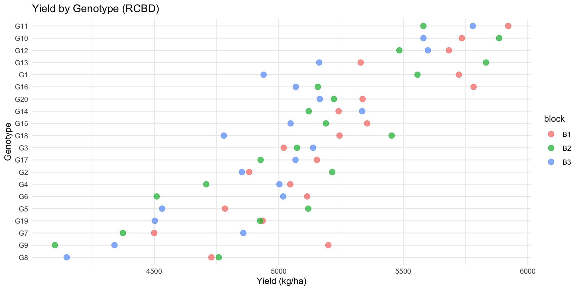
10 G18 5159. 345. 6.68# Visualization
ggplot(rcbd_data, aes(x = reorder(genotype, yield), y = yield, color = block)) +
geom_point(size = 3, alpha = 0.7) +
coord_flip() +
theme_minimal() +
labs(
title = "Yield by Genotype (RCBD)",
x = "Genotype",
y = "Yield (kg/ha)"
)
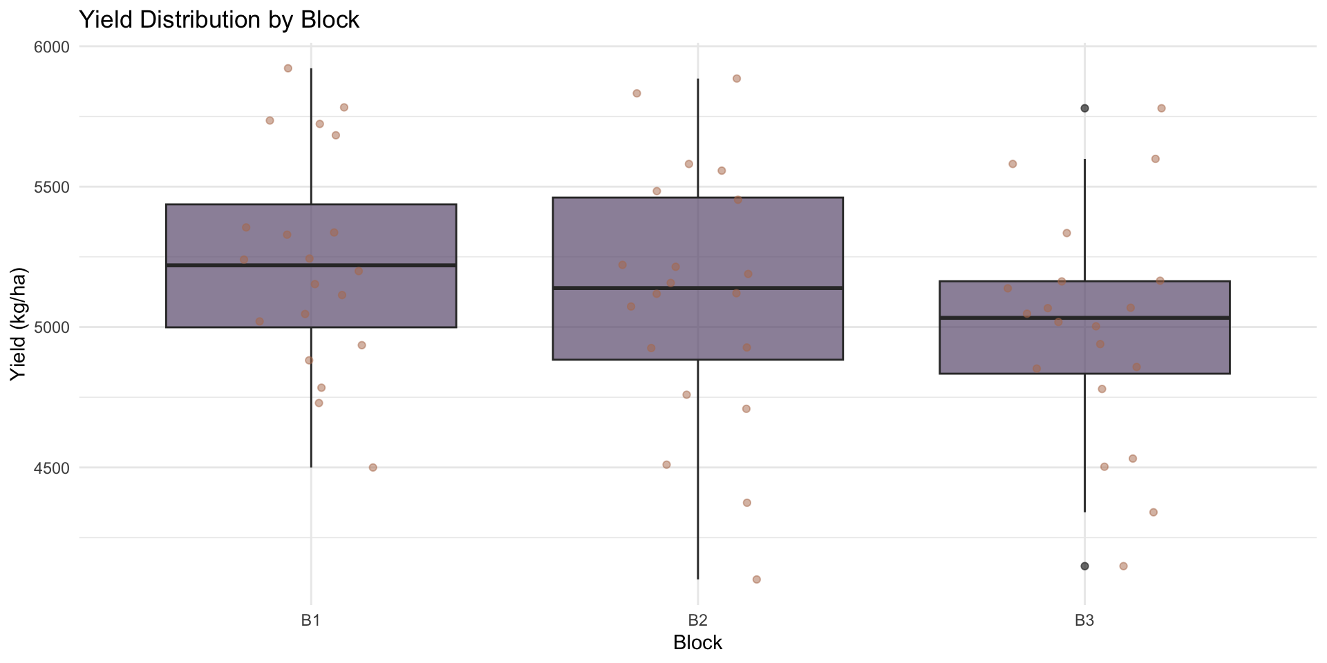
# Block effects
ggplot(rcbd_data, aes(x = block, y = yield)) +
  geom_boxplot(fill = "#6B5A7D", alpha = 0.7) +
  geom_jitter(width = 0.2, alpha = 0.5, color = "#B5795A") +
  theme_minimal() +
  labs(
    title = "Yield Distribution by Block",
    x = "Block",
    y = "Yield (kg/ha)"
  )
Model Fitting with Mandala
# Fit the RCBD model
rcbd_model <- mandala(
  fixed  = yield ~ genotype,
  random = ~ block,
  data   = rcbd_data
)
Initial data rows: 60
Final data rows after NA handling: 60 'as(<ddiMatrix>, "dgCMatrix")' is deprecated.
Use 'as(as(., "generalMatrix"), "CsparseMatrix")' instead.
See help("Deprecated") and help("Matrix-deprecated").--- Starting EM Warmup ---
EM Warmup: starting theta:
block 72640 R.sigma2 90800
EM iter 1: logLik=-292.7282; theta: block 50820 R.sigma2 43670
EM iter 2 : logLik decreased or failed. Stopping EM.
EM Warmup: ending theta:
block 50820 R.sigma2 43670
--- EM Warmup Complete. Starting AI-REML ---ai_reml_core(): method=autoStarting AI-REML logLik = -293.2461
Iter LogLik Sigma2 DF wall Restrained
1 -291.6739 54155.615 40 14:53:47 ( 0 restrained)
2 -291.1937 67152.963 40 14:53:47 ( 0 restrained)
3 -291.1899 70390.870 40 14:53:47 ( 0 restrained)
4 -291.1054 69557.565 40 14:53:47 ( 0 restrained)
5 -291.0187 67364.340 40 14:53:47 ( 0 restrained)
6 -290.9652 65521.102 40 14:53:47 ( 0 restrained)
7 -290.9408 64599.019 40 14:53:47 ( 0 restrained)
8 -290.9313 64451.096 40 14:53:47 ( 0 restrained)
9 -290.9270 64690.448 40 14:53:47 ( 0 restrained)
10 -290.9253 64991.927 40 14:53:47 ( 0 restrained)
11 -290.9248 65192.879 40 14:53:47 ( 0 restrained)
12 -290.9246 65267.209 40 14:53:47 ( 0 restrained)
13 -290.9245 65257.140 40 14:53:47 ( 0 restrained)
14 -290.9245 65215.852 40 14:53:47 ( 0 restrained)
15 -290.9245 65178.793 40 14:53:47 ( 0 restrained)
LogLik plateaued for 5 iterations -- stopping.
Main AI-REML Loop finished. Combining results.# View model summary and variance components
summary(rcbd_model)Model statement:
mandala(fixed = yield ~ genotype, random = ~block, data = rcbd_data)
Variance Components:
component estimate std.error z.ratio bound %ch
block 11206.94 14489.15 0.7734715 P NA
R.sigma2 65215.85 14971.01 4.3561411 P NA
Fixed Effects (BLUEs) [first 5]:
effect estimate std.error z.ratio
(Intercept) 5406.47680 159.6052 33.8740637
genotypeG10 327.20688 208.5108 1.5692566
genotypeG11 353.90274 208.5108 1.6972877
genotypeG12 182.19156 208.5108 0.8737754
genotypeG13 34.68584 208.5108 0.1663503
Converged: TRUE | Iterations: 15
Random Effects (BLUPs) [first 5]:
random level estimate std.error z.ratio
block B1 94.489529 73.61762 1.28351783
block B2 -3.138541 73.61762 -0.04263302
block B3 -91.348201 73.61762 -1.24084695
logLik: -290.925 AIC: 585.849 BIC: 589.227 logLik_Trunc: -254.167# Extract variance components table
var_components <- summary(rcbd_model)$varcompModel statement:
mandala(fixed = yield ~ genotype, random = ~block, data = rcbd_data)
Variance Components:
component estimate std.error z.ratio bound %ch
block 11206.94 14489.15 0.7734715 P NA
R.sigma2 65215.85 14971.01 4.3561411 P NA
Fixed Effects (BLUEs) [first 5]:
effect estimate std.error z.ratio
(Intercept) 5406.47680 159.6052 33.8740637
genotypeG10 327.20688 208.5108 1.5692566
genotypeG11 353.90274 208.5108 1.6972877
genotypeG12 182.19156 208.5108 0.8737754
genotypeG13 34.68584 208.5108 0.1663503
Converged: TRUE | Iterations: 15
Random Effects (BLUPs) [first 5]:
random level estimate std.error z.ratio
block B1 94.489529 73.61762 1.28351783
block B2 -3.138541 73.61762 -0.04263302
block B3 -91.348201 73.61762 -1.24084695
logLik: -290.925 AIC: 585.849 BIC: 589.227 logLik_Trunc: -254.167print(var_components) component estimate std.error z.ratio bound %ch
1 block 11206.94 14489.15 0.7734715 P NA
2 R.sigma2 65215.85 14971.01 4.3561411 P NA# Heritability Estimation
rcbd_model_rand <- mandala(
fixed = yield ~ 1,
random = ~ genotype + block,
data = rcbd_data
)Initial data rows: 60
Final data rows after NA handling: 60
--- Starting EM Warmup ---
EM Warmup: starting theta:
genotype 72640 block 72640 R.sigma2 90800
EM iter 1: logLik=-433.7394; theta: genotype 70060 block 50820 R.sigma2 75600
EM iter 2: logLik=-432.9942; theta: genotype 64280 block 36810 R.sigma2 88150
EM iter 3 : logLik decreased or failed. Stopping EM.
EM Warmup: ending theta:
genotype 64280 block 36810 R.sigma2 88150
--- EM Warmup Complete. Starting AI-REML ---ai_reml_core(): method=autoStarting AI-REML logLik = -433.4529
Iter LogLik Sigma2 DF wall Restrained
1 -432.2164 69766.090 59 14:53:47 ( 0 restrained)
2 -432.2091 53022.228 59 14:53:47 ( 0 restrained)
3 -432.2091 53022.228 59 14:53:47 ( 0 restrained)
Converged at iter 3 by tolerance(s): delta_theta=0.00e+00, delta_loglik=0.00e+00
Main AI-REML Loop finished. Combining results.h2_table <- h2_estimates(
random_mod = rcbd_model_rand,
fixed_mod = rcbd_model,
genotype = "genotype"
)
print(h2_table) variable value
source_random TRUE
source_fixed TRUE
sigma_g2 98837.0586124318
sigma_e2 53022.2280843937
n_rep 3
mean_PEV_BLUP 19185.1727994583
avsed_BLUE 208.511848912685
vdBLUE_avg 43477.1911369864
H2_Cullis 0.805890896908529
H2_Piepho 0.819709909797593
H2_Plot 0.650846324662066
H2_Standard 0.848305691274437
Note:
Plot and entry mean heritabilities are just the approximation- assuming a single experiment with only 'genotype' and 'error' variance components in the model. For MET, modify the equations and estimate accordingly# Extract adjusted genotype means (BLUEs) and rank genotypes
blue_means <- mandala_predict(rcbd_model, classify_term = "genotype")Random terms included: PEV matrix computed. Scale factor used = 1
Notes:
- The predictions are obtained by averaging across the hypertable
  calculated from model terms constructed solely from factors in
  the averaging and classify sets.
- The simple averaging set: (none)
- The ignored set: block
genotype_ranking <- blue_means %>% arrange(desc(predicted_value))
print(genotype_ranking) genotype predicted_value std_error
1 G11 5760.380 159.6065
2 G10 5733.684 159.6065
3 G12 5588.668 159.6065
4 G13 5441.163 159.6065
5 G1 5406.477 159.6052
6 G16 5335.982 159.6065
7 G20 5241.019 159.6065
8 G14 5231.767 159.6065
9 G15 5197.159 159.6065
10 G18 5158.919 159.6065
11 G3 5077.054 159.6065
12 G17 5049.098 159.6065
13 G2 4982.698 159.6065
14 G4 4919.307 159.6065
15 G6 4880.604 159.6065
16 G5 4811.351 159.6065
17 G19 4787.693 159.6065
18 G7 4577.274 159.6065
19 G9 4546.909 159.6065
20 G8 4545.699 159.6065Dataset 2: Alpha-Lattice Design
Data Description
An alpha-lattice design with:
- 50 genotypes
- 2 replications
- Incomplete blocks of size 5 within each replication
set.seed(789)
n_genotypes <- 50
n_reps <- 2
block_size <- 5
n_blocks_per_rep <- n_genotypes / block_size

# Create design structure
alpha_data <- data.frame(
  genotype = factor(rep(paste0("G", 1:n_genotypes), times = n_reps)),
  rep = factor(rep(1:n_reps, each = n_genotypes))
)

# Assign incomplete blocks within reps
alpha_data$incomplete_block <- factor(
  paste0(alpha_data$rep, ".",
         rep(rep(1:n_blocks_per_rep, each = block_size), times = n_reps))
)

# Simulate yield data
alpha_data$yield <- 6000

# Add genotype effects
genotype_effects <- rnorm(n_genotypes, mean = 0, sd = 400)
alpha_data$yield <- alpha_data$yield +
  genotype_effects[as.numeric(alpha_data$genotype)]

# Add rep effects
rep_effects <- c(300, -300)
alpha_data$yield <- alpha_data$yield +
  rep_effects[as.numeric(alpha_data$rep)]

# Add incomplete block effects
n_incomplete_blocks <- n_reps * n_blocks_per_rep
incomplete_block_effects <- rnorm(n_incomplete_blocks, mean = 0, sd = 200)
alpha_data$yield <- alpha_data$yield +
  incomplete_block_effects[as.numeric(alpha_data$incomplete_block)]

# Add error
alpha_data$yield <- alpha_data$yield + rnorm(nrow(alpha_data), mean = 0, sd = 350)

head(alpha_data, 10)
genotype rep incomplete_block yield
1 G1 1 1.1 6690.737
2 G2 1 1.1 6256.748
3 G3 1 1.1 6364.876
4 G4 1 1.1 6398.428
5 G5 1 1.1 6426.309
6 G6 1 1.2 5131.415
7 G7 1 1.2 7174.288
8 G8 1 1.2 6985.033
9 G9 1 1.2 6968.603
10 G10 1 1.2 4985.144Model Fitting
# Fit Alpha-Lattice Model
alpha_model_fixed <- mandala(
  fixed  = yield ~ genotype,
  random = ~ rep + rep:incomplete_block,
  data   = alpha_data
)
Initial data rows: 100
Final data rows after NA handling: 100
--- Starting EM Warmup ---
EM Warmup: starting theta:
rep 152000 rep:incomplete_block 152000 R.sigma2 190000
EM iter 1: logLik=-391.3152; theta: rep 137400 rep:incomplete_block 122500 R.sigma2 80030
EM iter 2 : logLik decreased or failed. Stopping EM.
EM Warmup: ending theta:
rep 137400 rep:incomplete_block 122500 R.sigma2 80030
--- EM Warmup Complete. Starting AI-REML ---ai_reml_core(): method=autoStarting AI-REML logLik = -391.4625
Iter LogLik Sigma2 DF wall Restrained
1 -388.9722 99238.374 50 14:53:47 ( 0 restrained)
2 -387.8479 123055.584 50 14:53:47 ( 0 restrained)
3 -387.6506 135005.966 50 14:53:47 ( 0 restrained)
4 -387.4433 136953.119 50 14:53:47 ( 0 restrained)
5 -387.2071 133881.113 50 14:53:47 ( 0 restrained)
6 -387.0147 129991.301 50 14:53:47 ( 0 restrained)
7 -386.8842 127391.733 50 14:53:47 ( 0 restrained)
8 -386.8012 126425.885 50 14:53:47 ( 0 restrained)
9 -386.7535 126551.856 50 14:53:47 ( 0 restrained)
10 -386.7357 127083.483 50 14:53:47 ( 0 restrained)
11 -386.7294 127562.203 50 14:53:47 ( 0 restrained)
12 -386.7272 127817.638 50 14:53:47 ( 0 restrained)
13 -386.7264 127872.012 50 14:53:47 ( 0 restrained)
14 -386.7260 127819.103 50 14:53:47 ( 0 restrained)
15 -386.7259 127743.357 50 14:53:47 ( 0 restrained)
16 -386.7259 127689.832 50 14:53:47 ( 0 restrained)
17 -386.7259 127668.121 50 14:53:47 ( 0 restrained)
LogLik plateaued for 5 iterations -- stopping.
Main AI-REML Loop finished. Combining results.summary(alpha_model_fixed)Model statement:
mandala(fixed = yield ~ genotype, random = ~rep + rep:incomplete_block,
data = alpha_data)
Variance Components:
component estimate std.error z.ratio bound %ch
rep 188544.87 272761.82 0.6912436 P NA
rep:incomplete_block 17666.16 21157.54 0.8349816 P NA
R.sigma2 127689.83 28564.28 4.4702621 P NA
Fixed Effects (BLUEs) [first 5]:
effect estimate std.error z.ratio
(Intercept) 6126.1006 408.5899 14.9932734
genotypeG10 -1212.1477 381.2500 -3.1794035
genotypeG11 184.7454 381.2500 0.4845780
genotypeG12 339.2113 381.2500 0.8897345
genotypeG13 -491.5735 381.2500 -1.2893729
Converged: TRUE | Iterations: 17
Random Effects (BLUPs) [first 5]:
random level estimate std.error z.ratio
rep 1 303.58093 310.4575 0.9778503
rep 2 -303.56283 310.4575 -0.9777921
rep:incomplete_block 1.1.1 19.31326 120.0306 0.1609028
rep:incomplete_block 1.1.10 -31.22415 120.0308 -0.2601344
rep:incomplete_block 1.1.2 36.17061 120.0308 0.3013443
logLik: -386.726 AIC: 779.452 BIC: 785.188 logLik_Trunc: -340.779var_comps_alpha <- summary(alpha_model_fixed)$varcompModel statement:
mandala(fixed = yield ~ genotype, random = ~rep + rep:incomplete_block,
data = alpha_data)
Variance Components:
component estimate std.error z.ratio bound %ch
rep 188544.87 272761.82 0.6912436 P NA
rep:incomplete_block 17666.16 21157.54 0.8349816 P NA
R.sigma2 127689.83 28564.28 4.4702621 P NA
Fixed Effects (BLUEs) [first 5]:
effect estimate std.error z.ratio
(Intercept) 6126.1006 408.5899 14.9932734
genotypeG10 -1212.1477 381.2500 -3.1794035
genotypeG11 184.7454 381.2500 0.4845780
genotypeG12 339.2113 381.2500 0.8897345
genotypeG13 -491.5735 381.2500 -1.2893729
Converged: TRUE | Iterations: 17
Random Effects (BLUPs) [first 5]:
random level estimate std.error z.ratio
rep 1 303.58093 310.4575 0.9778503
rep 2 -303.56283 310.4575 -0.9777921
rep:incomplete_block 1.1.1 19.31326 120.0306 0.1609028
rep:incomplete_block 1.1.10 -31.22415 120.0308 -0.2601344
rep:incomplete_block 1.1.2 36.17061 120.0308 0.3013443
logLik: -386.726 AIC: 779.452 BIC: 785.188 logLik_Trunc: -340.779print(var_comps_alpha) component estimate std.error z.ratio bound %ch
1 rep 188544.87 272761.82 0.6912436 P NA
2 rep:incomplete_block 17666.16 21157.54 0.8349816 P NA
3 R.sigma2 127689.83 28564.28 4.4702621 P NA# Heritability Estimation
alpha_model_random <- mandala(
fixed = yield ~ 1,
random = ~ genotype + rep + rep:incomplete_block,
data = alpha_data
)Initial data rows: 100
Final data rows after NA handling: 100
--- Starting EM Warmup ---
EM Warmup: starting theta:
genotype 152000 rep 152000 rep:incomplete_block 152000 R.sigma2 190000
EM iter 1: logLik=-766.1918; theta: genotype 133200 rep 137400 rep:incomplete_block 101600 R.sigma2 132300
EM iter 2: logLik=-762.6178; theta: genotype 115600 rep 126200 rep:incomplete_block 74720 R.sigma2 163200
EM iter 3: logLik=-762.2359; theta: genotype 104300 rep 117700 rep:incomplete_block 56690 R.sigma2 158300
EM iter 4: logLik=-761.4972; theta: genotype 95280 rep 111400 rep:incomplete_block 45080 R.sigma2 166600
EM iter 5: logLik=-761.3636; theta: genotype 88740 rep 106700 rep:incomplete_block 37040 R.sigma2 168800
EM Warmup: ending theta:
genotype 88740 rep 106700 rep:incomplete_block 37040 R.sigma2 168800
--- EM Warmup Complete. Starting AI-REML ---ai_reml_core(): method=autoStarting AI-REML logLik = -761.2430
Iter LogLik Sigma2 DF wall Restrained
1 -759.8962 138629.660 99 14:53:47 ( 0 restrained)
2 -759.6219 108637.486 99 14:53:47 ( 0 restrained)
3 -759.6219 108637.486 99 14:53:47 ( 0 restrained)
Converged at iter 3 by tolerance(s): delta_theta=0.00e+00, delta_loglik=0.00e+00
Main AI-REML Loop finished. Combining results.h2_alpha <- h2_estimates(
random_mod = alpha_model_random,
fixed_mod = alpha_model_fixed,
genotype = "genotype"
)
print(h2_alpha) variable value
source_random TRUE
source_fixed TRUE
sigma_g2 136443.111750374
sigma_e2 108637.485589384
n_rep 2
mean_PEV_BLUP 44650.149532677
avsed_BLUE 379.359551187455
vdBLUE_avg 143913.669077147
H2_Cullis 0.672756294107645
H2_Piepho 0.654717595565955
H2_Plot 0.556727514260222
H2_Standard 0.715253644790606
Note:
Plot and entry mean heritabilities are just the approximation- assuming a single experiment with only 'genotype' and 'error' variance components in the model. For MET, modify the equations and estimate accordingly# BLUPs
blups_alpha <- mandala_predict(alpha_model_random, classify_term = "genotype")Random terms included: PEV matrix computed. Scale factor used = 108637
Notes:
- The predictions are obtained by averaging across the hypertable
  calculated from model terms constructed solely from factors in
  the averaging and classify sets.
- The simple averaging set: (none)
- The ignored set: rep, rep:incomplete_blockhead(blups_alpha) genotype predicted_value std_error
1 G1 6060.863 117035.9
2 G10 5228.278 117035.9
3 G11 6197.783 117035.9
4 G12 6308.265 117035.9
5 G13 5714.043 117035.9
6 G14 6053.733 117035.9Dataset 3: Multi-Environment Trial
Data Description
A multi-environment trial with:
- 30 genotypes
- 4 locations (environments)
- 3 blocks per location
set.seed(101)
n_genotypes <- 30
n_locations <- 4
n_blocks <- 3

met_data <- expand.grid(
  genotype = factor(paste0("G", 1:n_genotypes)),
  location = factor(paste0("Loc", 1:n_locations)),
  block = factor(paste0("B", 1:n_blocks))
)

# Simulate yield data
met_data$yield <- 5500

# Add genotype main effects
genotype_effects <- rnorm(n_genotypes, mean = 0, sd = 300)
met_data$yield <- met_data$yield +
  genotype_effects[as.numeric(met_data$genotype)]

# Add location effects
location_effects <- c(800, 200, -300, -700)
met_data$yield <- met_data$yield +
  location_effects[as.numeric(met_data$location)]

# Add genotype x location interaction
gxe_effects <- matrix(
  rnorm(n_genotypes * n_locations, mean = 0, sd = 250),
  nrow = n_genotypes,
  ncol = n_locations
)
met_data$yield <- met_data$yield +
  gxe_effects[cbind(as.numeric(met_data$genotype),
                    as.numeric(met_data$location))]

# Add block within location effects
n_block_loc <- n_locations * n_blocks
block_loc_effects <- rnorm(n_block_loc, mean = 0, sd = 150)
met_data$block_loc <- factor(paste0(met_data$location, "_", met_data$block))
met_data$yield <- met_data$yield +
  block_loc_effects[as.numeric(met_data$block_loc)]

# Add error
met_data$yield <- met_data$yield + rnorm(nrow(met_data), mean = 0, sd = 400)

head(met_data, 10)
genotype location block yield block_loc
1 G1 Loc1 B1 5731.465 Loc1_B1
2 G2 Loc1 B1 5523.519 Loc1_B1
3 G3 Loc1 B1 5900.409 Loc1_B1
4 G4 Loc1 B1 6928.250 Loc1_B1
5 G5 Loc1 B1 5208.988 Loc1_B1
6 G6 Loc1 B1 5877.214 Loc1_B1
7 G7 Loc1 B1 6453.261 Loc1_B1
8 G8 Loc1 B1 5900.387 Loc1_B1
9 G9 Loc1 B1 6430.253 Loc1_B1
10 G10 Loc1 B1 6269.523 Loc1_B1Exploratory Analysis
# Location summary
met_data %>%
  group_by(location) %>%
  summarise(
    mean_yield = mean(yield),
    sd_yield = sd(yield),
    min_yield = min(yield),
    max_yield = max(yield)
  )
# A tibble: 4 × 5
location mean_yield sd_yield min_yield max_yield
<fct> <dbl> <dbl> <dbl> <dbl>
1 Loc1 6156. 488. 4924. 7290.
2 Loc2 5567. 605. 4126. 6960.
3 Loc3 5304. 536. 4058. 6528.
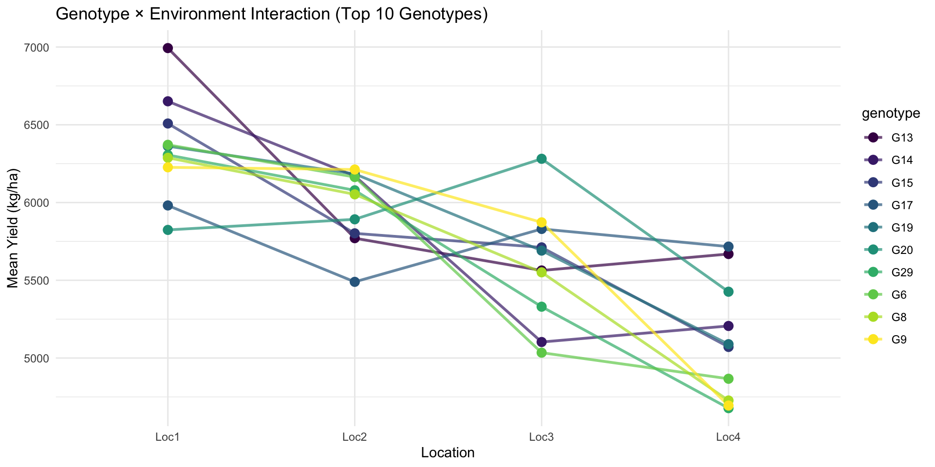
4 Loc4 4686. 545. 3584. 6042.# GxE interaction plot
met_means <- met_data %>%
group_by(genotype, location) %>%
summarise(mean_yield = mean(yield), .groups = "drop")
# Select top 10 genotypes for visualization
top_genotypes <- met_means %>%
group_by(genotype) %>%
summarise(overall_mean = mean(mean_yield), .groups = "drop") %>%
arrange(desc(overall_mean)) %>%
head(10) %>%
pull(genotype)
met_means %>%
filter(genotype %in% top_genotypes) %>%
ggplot(aes(x = location, y = mean_yield, group = genotype, color = genotype)) +
geom_line(linewidth = 1, alpha = 0.7) +
geom_point(size = 3) +
theme_minimal() +
scale_color_viridis_d() +
labs(
title = "Genotype × Environment Interaction (Top 10 Genotypes)",
x = "Location",
y = "Mean Yield (kg/ha)"
)
Model Fitting
# Fit Multi-Environment Model
met_model_fixed <- mandala(
  fixed  = yield ~ genotype + location + genotype:location,
  random = ~ location:block,
  data   = met_data
)
Initial data rows: 360
Final data rows after NA handling: 360
--- Starting EM Warmup ---
EM Warmup: starting theta:
location:block 229700 R.sigma2 287100
EM iter 1: logLik=-1865.5855; theta: location:block 160600 R.sigma2 98970
EM iter 2: logLik=-1849.9651; theta: location:block 115600 R.sigma2 99410
EM iter 3: logLik=-1848.8735; theta: location:block 84830 R.sigma2 99180
EM iter 4: logLik=-1848.3127; theta: location:block 64240 R.sigma2 99260
EM iter 5: logLik=-1847.8266; theta: location:block 50430 R.sigma2 99350
EM Warmup: ending theta:
location:block 50430 R.sigma2 99350
--- EM Warmup Complete. Starting AI-REML ---ai_reml_core(): method=autoStarting AI-REML logLik = -1847.5449
Iter LogLik Sigma2 DF wall Restrained
1 -1840.3336 123189.367 240 14:53:48 ( 0 restrained)
2 -1839.3973 152754.815 240 14:53:48 ( 0 restrained)
3 -1839.3973 152754.815 240 14:53:48 ( 0 restrained)
Converged at iter 3 by tolerance(s): delta_theta=0.00e+00, delta_loglik=0.00e+00
Main AI-REML Loop finished. Combining results.summary(met_model_fixed)Model statement:
mandala(fixed = yield ~ genotype + location + genotype:location,
random = ~location:block, data = met_data)
Variance Components:
component estimate std.error z.ratio bound %ch
location:block 40270.0 22191.43 1.814664 P NA
R.sigma2 152754.8 11437.85 13.355209 P NA
Fixed Effects (BLUEs) [first 5]:
effect estimate std.error z.ratio
(Intercept) 5968.0741 253.6442 23.5293175
genotypeG10 607.3811 319.1079 1.9033724
genotypeG11 300.6162 319.1079 0.9420520
genotypeG12 163.7220 319.1079 0.5130616
genotypeG13 1025.1174 319.1079 3.2124481
Converged: TRUE | Iterations: 3
Random Effects (BLUPs) [first 5]:
random level estimate std.error z.ratio
location:block Loc1.B1 -25.31215 128.2062 -0.1974332
location:block Loc2.B1 302.57897 128.2062 2.3600960
location:block Loc3.B1 -42.51595 128.2062 -0.3316216
location:block Loc4.B1 -15.29247 128.2062 -0.1192803
location:block Loc1.B2 116.55314 128.2062 0.9091071
logLik: -1839.397 AIC: 3682.795 BIC: 3689.756 logLik_Trunc: -1618.852var_comps_met <- summary(met_model_fixed)$varcompModel statement:
mandala(fixed = yield ~ genotype + location + genotype:location,
random = ~location:block, data = met_data)
Variance Components:
component estimate std.error z.ratio bound %ch
location:block 40270.0 22191.43 1.814664 P NA
R.sigma2 152754.8 11437.85 13.355209 P NA
Fixed Effects (BLUEs) [first 5]:
effect estimate std.error z.ratio
(Intercept) 5968.0741 253.6442 23.5293175
genotypeG10 607.3811 319.1079 1.9033724
genotypeG11 300.6162 319.1079 0.9420520
genotypeG12 163.7220 319.1079 0.5130616
genotypeG13 1025.1174 319.1079 3.2124481
Converged: TRUE | Iterations: 3
Random Effects (BLUPs) [first 5]:
random level estimate std.error z.ratio
location:block Loc1.B1 -25.31215 128.2062 -0.1974332
location:block Loc2.B1 302.57897 128.2062 2.3600960
location:block Loc3.B1 -42.51595 128.2062 -0.3316216
location:block Loc4.B1 -15.29247 128.2062 -0.1192803
location:block Loc1.B2 116.55314 128.2062 0.9091071
logLik: -1839.397 AIC: 3682.795 BIC: 3689.756 logLik_Trunc: -1618.852print(var_comps_met) component estimate std.error z.ratio bound %ch
1 location:block 40270.0 22191.43 1.814664 P NA
2 R.sigma2 152754.8 11437.85 13.355209 P NA# Heritability Estimation
met_model_random <- mandala(
fixed = yield ~ location,
random = ~ genotype + genotype:location + location:block,
data = met_data
)Initial data rows: 360
Final data rows after NA handling: 360
--- Starting EM Warmup ---
EM Warmup: starting theta:
genotype 229700 genotype:location 229700 location:block 229700 R.sigma2 287100
EM iter 1: logLik=-2754.0859; theta: genotype 155400 genotype:location 162300 location:block 160600 R.sigma2 142100
EM iter 2: logLik=-2715.4535; theta: genotype 111900 genotype:location 126100 location:block 115600 R.sigma2 155600
EM iter 3: logLik=-2710.1406; theta: genotype 84090 genotype:location 99910 location:block 84970 R.sigma2 151200
EM iter 4: logLik=-2705.7996; theta: genotype 66500 genotype:location 82520 location:block 64480 R.sigma2 154500
EM iter 5: logLik=-2704.0857; theta: genotype 55100 genotype:location 70520 location:block 50680 R.sigma2 156500
EM Warmup: ending theta:
genotype 55100 genotype:location 70520 location:block 50680 R.sigma2 156500
--- EM Warmup Complete. Starting AI-REML ---ai_reml_core(): method=autoStarting AI-REML logLik = -2703.5430
Iter LogLik Sigma2 DF wall Restrained
1 -2702.7530 144938.837 356 14:53:49 ( 0 restrained)Warning in ai_reml_core(y = y, X = X, Zlst = built_G$Zlst, random_names =
built_G$random_names, : Iter 2: Fast step rejected. Re-using previous
parameters. 2 -2702.7530 144938.837 356 14:53:49 ( 0 restrained)
Converged at iter 2 by tolerance(s): delta_theta=0.00e+00, delta_loglik=0.00e+00
Main AI-REML Loop finished. Combining results.h2_met <- h2_estimates(
random_mod = met_model_random,
fixed_mod = met_model_fixed,
genotype = "genotype"
)
print(h2_met) variable value
source_random TRUE
source_fixed TRUE
sigma_g2 63388.6139119626
sigma_e2 144938.837455179
n_rep 12
mean_PEV_BLUP 21224.4944796125
avsed_BLUE 559.483573688463
vdBLUE_avg 313021.869227213
H2_Cullis 0.665168660903514
H2_Piepho 0.288261682831932
H2_Plot 0.304273937476685
H2_Standard 0.83995308674032
Note:
Plot and entry mean heritabilities are just the approximation- assuming a single experiment with only 'genotype' and 'error' variance components in the model. For MET, modify the equations and estimate accordingly# BLUPs
blups_by_loc <- mandala_predict(met_model_random, classify_term = "genotype:location")Random terms included: PEV matrix computed. Scale factor used = 1
Notes:
- The predictions are obtained by averaging across the hypertable
  calculated from model terms constructed solely from factors in
  the averaging and classify sets.
- The simple averaging set: (none)
- The ignored set: location:block
blups_overall <- mandala_predict(met_model_random, classify_term = "genotype")Random terms included:
PEV matrix computed. Scale factor used = 1
Notes:
- The predictions are obtained by averaging across the hypertable
  calculated from model terms constructed solely from factors in
  the averaging and classify sets.
- The simple averaging set: location, [num mean]
- The ignored set: location:blockhead(blups_overall) genotype predicted_value std_error
1 G1 5345.805 118.5263
2 G10 5386.511 118.5263
3 G11 5178.997 118.5263
4 G12 5529.319 118.5263
5 G13 5924.195 118.5263
6 G14 5736.369 118.5263Summary
This tutorial demonstrated:
- RCBD Analysis — Simple randomized complete block design
- Alpha-Lattice Design — Incomplete block designs
- Multi-Environment Trials — Analyzing GxE interactions
Next Steps
Session Information
sessionInfo()R version 4.5.2 (2025-10-31)
Platform: aarch64-apple-darwin20
Running under: macOS Tahoe 26.1
Matrix products: default
BLAS: /System/Library/Frameworks/Accelerate.framework/Versions/A/Frameworks/vecLib.framework/Versions/A/libBLAS.dylib
LAPACK: /Library/Frameworks/R.framework/Versions/4.5-arm64/Resources/lib/libRlapack.dylib; LAPACK version 3.12.1
locale:
[1] C.UTF-8/C.UTF-8/C.UTF-8/C/C.UTF-8/C.UTF-8
time zone: America/New_York
tzcode source: internal
attached base packages:
[1] stats graphics grDevices utils datasets methods base
other attached packages:
[1] tidyr_1.3.1 ggplot2_4.0.0 dplyr_1.1.4 mandala_1.1.0
loaded via a namespace (and not attached):
[1] Matrix_1.7-4 gtable_0.3.6 jsonlite_2.0.0 compiler_4.5.2
[5] tidyselect_1.2.1 Rcpp_1.1.0 splines2_0.5.4 scales_1.4.0
[9] yaml_2.3.10 fastmap_1.2.0 lattice_0.22-7 R6_2.6.1
[13] labeling_0.4.3 generics_0.1.4 knitr_1.50 htmlwidgets_1.6.4
[17] tibble_3.3.0 pillar_1.11.1 RColorBrewer_1.1-3 rlang_1.1.6
[21] utf8_1.2.6 xfun_0.54 S7_0.2.0 viridisLite_0.4.2
[25] cli_3.6.5 withr_3.0.2 magrittr_2.0.4 digest_0.6.37
[29] grid_4.5.2 lifecycle_1.0.4 vctrs_0.6.5 evaluate_1.0.5
[33] glue_1.8.0 farver_2.1.2 codetools_0.2-20 rmarkdown_2.30
[37] purrr_1.1.0 tools_4.5.2 pkgconfig_2.0.3 htmltools_0.5.8.1